Generative Adversarial Networks (GANs)

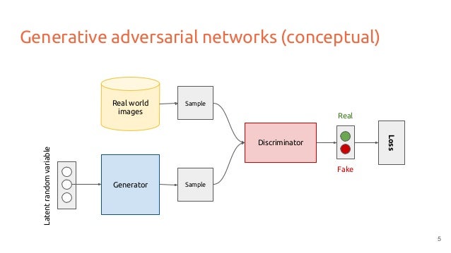
The GAN concept solves the problem of training a generative network ($//<![CDATA[ \begin{array}{l}G\end{array} //]]>$) by introducing a second discriminative network ($//<![CDATA[ \begin{array}{l}D\end{array} //]]>$). The setup is referred to as adversarial, since $//<![CDATA[ \begin{array}{l}D\end{array} //]]>$ and $//<![CDATA[ \begin{array}{l}G\end{array} //]]>$ are in a constant battle against each other, as illustrated in figure 1. While $//<![CDATA[ \begin{array}{l}G\end{array} //]]>$ tries to create increasingly more realistic images to fool $//<![CDATA[ \begin{array}{l}D\end{array} //]]>$, $//<![CDATA[ \begin{array}{l}D\end{array} //]]>$ is constantly adapting its parameters to make a more informed decision. As figure 2 shows, this yields two scenarios: On the left, a real image is shown to $//<![CDATA[ \begin{array}{l}D\end{array} //]]>$ directly and $//<![CDATA[ \begin{array}{l}D\end{array} //]]>$ tries to classify it as real as confidently as possible. On the right, an image is generated by $//<![CDATA[ \begin{array}{l}G\end{array} //]]>$ and then shown to $//<![CDATA[ \begin{array}{l}D\end{array} //]]>$. While $//<![CDATA[ \begin{array}{l}D\end{array} //]]>$ tries to drive its prediction of real on the generated image to 0, $//<![CDATA[ \begin{array}{l}G\end{array} //]]>$ tries to push it into the opposite direction by creating more realistic images.

In the original setup introduced by Goodfellow et al. ⁽¹⁾, fully connected layers were used for both $//<![CDATA[ \begin{array}{l}D\end{array} //]]>$ and $//<![CDATA[ \begin{array}{l}G\end{array} //]]>$. However, the usage of convolutional layers showed even greater potential and is the current state-of-the-art ⁽²⁾.

The setup can be interpreted as a zero-sum game within game theory, which follows a min-max character. On the one hand, $//<![CDATA[ \begin{array}{l}D\end{array} //]]>$ tries to maximize the probability of correctly distinguishing between real and fake data by changing its decision boundary. On the other hand, $//<![CDATA[ \begin{array}{l}G\end{array} //]]>$ tries to minimize the probability of its generated samples being classified as fake.

The outcome of the game is fed back to both networks using back-propagation. This allows both networks to iteratively improve their policy on how to decide and act within their respective tasks.

In terms of game theory, training a GAN requires finding Nash equilibria in high-dimensional, continuous, non-convex games. This is an incredibly hard task with no clear solution strategy to it.

Mathematically, the dataset of real images is a number of examples drawn from a true data distribution, which is shown in blue in figure 3. $//<![CDATA[ \begin{array}{l}G\end{array} //]]>$ takes a code as an input, e.g., taken from a unit Gaussian distribution $//<![CDATA[ \begin{array}{l}z\end{array} //]]>$, and tries to generate a distribution $//<![CDATA[ \begin{array}{l}\hat p(x)\end{array} //]]>$ similar to the true distribution $//<![CDATA[ \begin{array}{l}p(x)\end{array} //]]>$. $//<![CDATA[ \begin{array}{l}G\end{array} //]]>$ is constantly trying to adjust its parameters $//<![CDATA[ \begin{array}{l}\theta\end{array} //]]>$ to stretch and squeeze the input to better match the true distribution.

Figure 4 gives us a good impression how $//<![CDATA[ \begin{array}{l}G\end{array} //]]>$ tries to fit its distribution to the true distribution (black dots) while $//<![CDATA[ \begin{array}{l}D\end{array} //]]>$ adapts the decision boundary to best distinguish between the generated and real data. We see in (a) the initial setup, (b) where $//<![CDATA[ \begin{array}{l}D\end{array} //]]>$ has updated its decision boundary, (c) where $//<![CDATA[ \begin{array}{l}G\end{array} //]]>$ has updated its distribution by shifting into the same direction as $//<![CDATA[ \begin{array}{l}D\end{array} //]]>$ has shifted its decision boundary, and finally (d) where we have reached the final equilibrium where $//<![CDATA[ \begin{array}{l}G\end{array} //]]>$ is perfectly mimicking the true data distribution and $//<![CDATA[ \begin{array}{l}D\end{array} //]]>$ can only decide randomly, indicated by the uniform decision boundary.

Figure 1: GAN concept: $//<![CDATA[ \begin{array}{l}D\end{array} //]]>$ tries to correctly detect, if images came from real world examples or $//<![CDATA[ \begin{array}{l}G\end{array} //]]>$. $//<![CDATA[ \begin{array}{l}G\end{array} //]]>$ as the adversary tries to improve its image generation to fool $//<![CDATA[ \begin{array}{l}D\end{array} //]]>$.  Source: Link

Figure 2: Two scenarios: On the left, training examples $//<![CDATA[ \begin{array}{l}x\end{array} //]]>$ are randomly sampled from the training set and used as input for $//<![CDATA[ \begin{array}{l}D\end{array} //]]>$. On the right, inputs $//<![CDATA[ \begin{array}{l}z\end{array} //]]>$ to $//<![CDATA[ \begin{array}{l}G\end{array} //]]>$ are randomly sampled from the model’s prior over the latent variables. $//<![CDATA[ \begin{array}{l}D\end{array} //]]>$ then receives input $//<![CDATA[ \begin{array}{l}G(z)\end{array} //]]>$, a fake sample created by $//<![CDATA[ \begin{array}{l}G\end{array} //]]>$.  Source: (7)

Figure 3: Representation of distribution space.  Source: (8)

Figure 4: Evolution of $//<![CDATA[ \begin{array}{l}G\end{array} //]]>$'s distribution (green) and the $//<![CDATA[ \begin{array}{l}D\end{array} //]]>$'s decision boundary (blue).  Source: (1)

A big breakthrough in the research about GANs has been achieved through the Deep Convolutional GAN (DCGAN) by Radford et al. ⁽²⁾ who applied a list of empirically validated tricks as the substitution of pooling and fully connected layers with convolutional layers. For $//<![CDATA[ \begin{array}{l}G\end{array} //]]>$, a fractional stride was utilized while $//<![CDATA[ \begin{array}{l}D\end{array} //]]>$ used integer stride. The network takes 100 random numbers drawn from a uniform distribution (the so-called code or latent variables) as an input. The generator network then creates a 64x64 color image.

By changing the code incrementally, we observe meaningful changes in the generated images, while remaining real-looking. This is a clear sign that the network has learned actual representation or features of how the world looks like and it has encoded this information in the network.

The procedure of incrementally changing parts of the input code is described as walking in the latent space. As an example, we could perform a stepwise interpolation between two codes and see how the result changes. One experiment in the DCGAN publication ⁽²⁾ trained a network on images of bedrooms. An interpolation between the code of two different bedrooms showed how the rooms are slowly transforming while constantly keeping the look of a bedroom. In figure 5 we can observe lamps turning into windows (first row) or a TV transforming into a large window (last row).

Another evidence that the network has learned representations can be found in visualizing the filters of the network in figure 6. We can clearly see that the untrained, random filters look almost like a single sample picture. However, the trained filters have clearly discovered features that are significant for a bedroom.

Another remarkable observation is that the input codes support vector arithmetic. This means if we take, e.g., the averaged code of three smiling women, subtract neutral women, add neutral men and then feed the resulting code through the network, we get a smiling man (as shown in figure 7).

Figure 4: DCGAN generator: A series of fractionally-strided convolutions convert the input vector (code) into an image ($//<![CDATA[ \begin{array}{l}G(z)\end{array} //]]>$) Source: created from (7)

The power of the features encoded in the latent variables was further explored by Chen at al. ⁽⁴⁾. They made use of the fact that the latent space of a regular GAN is underspecified to add additional input parameters (referred to as extend code) and thereby functionality. They decomposed the code in the latent code seen before and an additional latent component, which targets the semantic features of the data distribution. The goal is to learn disentangled and interpretable representations.

This is achieved by maximizing the mutual information between small subsets of the representation variables and observations. Therefore, Chen at al. introduced a regularization term that gives weight to an entropy based indicator of how much information is shared between the latent code and the generated distribution.

The publication showed remarkable results. In the MNIST ⁽¹⁰⁾. dataset the digit type, rotation, and width of the digits was captured in separate designated parts of the additional latent component. On a 3D faces data set the azimuth, elevation, lighting, and the width of the face were captured and identified.

GANs have also been used in the field of semi-supervised learning, where a small amount of labeled data is combined with a large amount of unlabeled data. In this setting, $//<![CDATA[ \begin{array}{l}D\end{array} //]]>$ is a classifier with output dimension of $//<![CDATA[ \begin{array}{l}n+1\end{array} //]]>$ that gives weight to the $//<![CDATA[ \begin{array}{l}n\end{array} //]]>$ classes to be identified plus a variable indicating if the image is real or not.

This allows the classifier to be additionally trained with unlabeled data which is known to be real, and with samples from the generator, which are known to be fake.

Through this approach, named feature matching GANs, good performance on the MNIST data set can be achieved with as little as 20 labeled training examples. ⁽³⁾

Figure 8: Manipulating latent codes on MNIST. Source: (4)