Batch Normalization - Algorithm
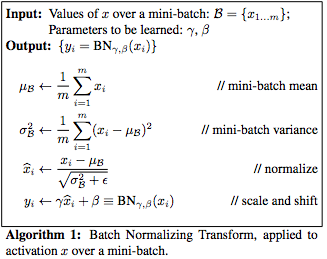
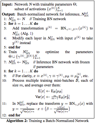
Batch normalization (BN) consists of two algorithms. Algorithm 1 is the transformation of the original input of a layer x to the shifted and normalized value y. Algorithm 2 is the overall training of a batch-normalized network.
In both algorithms, the value ε is inserted to avoid dividing by 0 and is selected to be insignificant small (e.g.~10(-8)) on purpose.
Algortihm 1 uses the following simplification:
- The scalar features are normalized independently, making their means 0 and the variance 1. This means in case of a d-dimensional input x = {x(1)…x(d)}, each dimension of the input x is normalized independently, thus every variable x, y, μ, σ becomes x(k), y(k), μ (k), σ(k).
- Each mini-batch produces estimates of the mean and variance of each activation. This ensures that a batch-normalized network retains its ability to fully use backpropagation.
As a simple normalization of x, as demonstrated in at the third step of Algroitm 1, may lead to a change of the representation of the affected layer, y is introduced. The introduction of y makes sure that the transformation represents an identity transform, meaning that x is fully substituted by y for every input. Thus γ and β are introduced as scale and shift parameters, which are to be learned besides the already existing parameters of the network (as seen in Algorithm 1 Step 4). This increases the amount of parameters to be learned, but the BN compensations that with an increase regarding the learning speed and overall fewer processing steps. Note that γ and β also become γ(k) and β(k) in the case of d-dimensional input.
Since the normalization of the scalars is done independently, the use of the mini-patches can be done without special means or additional transformation. If the scalars were jointly normalized, further regulations would be required, resulting from the likely smaller size of the mini-patches compared to the number of normalized actions, leading to a singular covariance matrices.
As mentioned, BN can fully partake in the process of backproporgation. The resulting operations for the variables of BN transformation are as follows:
\frac{\partial l}{\partial \hat{x}_i} = \frac{\partial l}{\partial y_i} \cdot \gamma
\\
\frac{\partial l}{\partial \sigma_B^2} = \sum_{i=1}^m \frac{\partial l}{\partial \hat{x}_i} \cdot (x_i - \mu_B) \cdot \frac{-1}{2}(\sigma_B^2 + \epsilon)^{\frac{-3}{2}}
\\
\frac{\partial l}{\partial \mu_B} = \left( \sum_{i=1}^m \frac{\partial l}{\partial \hat{x}_i} \cdot \frac{-1}{\sqrt{\sigma_B^2 + \epsilon}}\right) +\frac{\partial l}{\partial \sigma_B^2} \cdot \frac{\sum_{i=1}^m -2(x_i -\mu_B)}{m}
\\
\frac{\partial l}{\partial x_i} = \frac{\partial l}{\partial \hat{x}_i} \cdot \frac{-1}{\sqrt{\sigma_B^2 + \epsilon}} + \frac{\partial l}{\partial \sigma_B^2} \cdot \frac{2(x_i - \mu_B)}{m} + \frac{\partial l}{\partial \sigma_B^2} \cdot \frac{1}{m}
\\
\frac{\partial l}{\partial \gamma} = \sum_{i=1}^m \frac{\partial l}{\partial y_i} \cdot \hat{x}_i
\\
\frac{\partial l }{\partial \beta} = \sum_{i=1}^m \frac{\partial l}{\partial y_i}
Algorithm 2 has in essence three parts:
- Step 1 to 5 is to transform the network into an BN network using Algorithm 1
- Step 6 to 7 is the training of the new network,
- Step 8 to 12 is to transform the batch statistic into a population statistic.
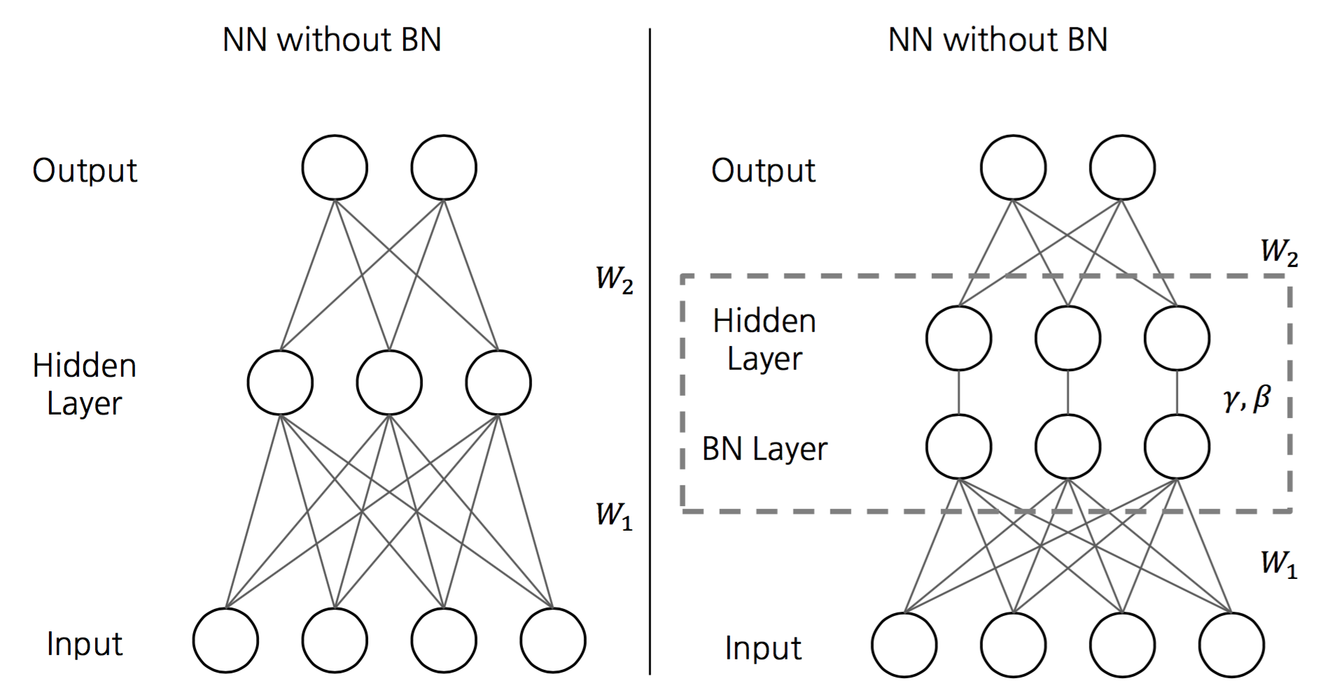
 Figure 1: (3) Comparison of a neural network with and without a BN step.
The BN is performed before the other processes of the network in this layer are applied, as is visualized in Figure 1. Any kind of batch gradient descent, Stochastic Gradient Descent and its variants can be applied to train the BN network.
In case of non-linear operations, such as ReLU, the BN transformation has to be applied before the non-linear operation. Assume a model z = g(Wu +B), with W and b being the parameters the model learned, g(.) being the nonlinear transformation and u being the input. Thus it becomes z = g(BN(Wu)), with \beta of the BN taking over the role of the bias b.
Due to the normalization of every action in the network, additional benefits to the hindrance to the internal covariance shift are achieved. BN transformation makes the network parameters scale-invariant, meaning BN(WU) = BN((aW)u), using scalar a. It can further be shown that the scale also does not affect the Jacobian of the respective layer nor the gradient propagation, meaning
|
\frac{\partial BN((aW)u)}{\partial u} = \frac{\partial BN(Wu)}{u}
\\
\frac{\partial BN((aW)u)}{\partial aW} = \frac{1}{a} \cdot \frac{\partial BN(Wu)}{\partial W} |
Due to the normalization, the BN further prevents smaller changes to the parameters to amplify and thereby allows higher learning rates, making the network even faster.
In order to use BN for convolutional layers, the two algorithms must be adjusted. The mini-batch B in Algorithm 1 must be per feature map, leading to mini-batch size of m' = m \cdot pq, with a feature map of size p \times q. Thus the parameters \gamma^{(k)} and \beta^{(k)} are collected per feature map, not per activation. This also applies to Algorithm 2.


2 Kommentare
Unbekannter Benutzer (ga29mit) sagt:
26. Januar 2017All the comments are SUGGESTIONS and are obviously highly subjective!
Form comments:
Wording comments:
Corrections:
In the case that the input distribution of a learning system, such as a neural network, changes, one speaks of a so-called covariate shift.
If this change happens on the input of internal nodes of (deep) neural networks, it is called an internal covariate shift.
assume there exist two conditional distributions
To counteract this, re-training of the network with a weighting of the data of the source by Pt(X)/Ps(X), or similar technics, are to be applied.
To counteract this, re-training of the network with a weighting of the data of the source by Pt(X)/Ps(X), or similar technics, have to be applied.
faulty data distribution, the aforementioned internal covariate shift.
faulty data distribution, due to the aforementioned internal covariate shift.
if deep learning is to be used, this must be addressed.
if deep learning is used, this has to be addressed.
The algorithm 1 is the
Algorithm 1 is the
The algorithm 2 is the
Algorithm 2 is the
making its means 0 and the variance 1.
making their means 0 and the variance 1.
This ensures, that an batch-normalized network
This ensures that a batch-normalized network
As a simple normalization of x, as writen in Algorithm 1 Step 3, may lead to an change of the representation of the affected layer, y is introduced to make sure, that the transformation represents an identity transform, meaning every input, which would have originaly reseved x now gets y.
Since a simple normalization of x, as demonstrated in Algorithm 1 Step 3, may lead to a change of the representation of the affected layer, y is introduced. The introduction of y makes sure that the transformation represents an identity transform, meaning that x is fully substituted by y for every input.
γ(k) and β(k) in case of d-demensional input.
γ(k) and β(k) in the case of d-dimensional input.
use of the mini-patches can done without special means or aditional transforamtion
use of the mini-patches can be done without special means or additional transformation
Would the scalars be jointly normalized, further regulations would be required, resulting from the likly smaller size of the mini-patches compared to the number of normalized actions, meaning in a singular covariance matrices.
If the scalars were jointly normalized, further regulations would be required, resulting from the likely smaller size of the mini-patches compared to the number of normalization actions, leading to singular covariance matrices.
The BN is performed, before the other processes of the network in this layer are applied, as is visulized in Figure 1
The BN is performed before the other processes of the network in this layer are applied, as is visualized in Figure 1
Due to the normalization of every action in the network, additional benefitts to the hindrance to the internal covariance shift are achieed.
Due to the normalization of every action in the network, additional benefits to the hindrance to the internal covariance shift are achieved.
The BN further prevents smaller changes to the parameters to amplify, due to the normalization, thus allowing higher learning rates, making the network even faster.
Due to the normalization, the BN further prevents smaller changes to the parameters to amplify and thereby allows higher learning rates, making the network even faster.
with a feature map the size p×q p×q.
with a feature map of size p×q p×q.
Thus the parameters γ(k) and β(k) are per feature map, not per activation
Thus the parameters γ(k) and β(k) are collected per feature map, not per activation
Unbekannter Benutzer (ga73fuj) sagt:
30. Januar 2017General suggestions:
Corrections: