Applications in which the training data comprises examples of the input vectors along with their corresponding target vectors are known as supervised learning problems[1]. The training data consists of a set of training examples. In supervised learning, each example is a pair consisting of an input object(typically a vector) and a desired output value (also called the supervisory signal).For instance, a training example in neural network could be like this,
| (1) | (\vec{x}_i, \vec{y}_i), 0<i\leq n |
, where \vec{x}_i is the i^{th} input vector and correspondingly \vec{y}_i is the desired i^{th} output vector.
Error Measures
What we'd like during learning process is an algorithm which let us find weights and biases so that the output from the network \vec{f}(\vec{x}_i) approximates \vec{y}_i for all training inputs \vec{x}_i. To quantify how well we're achieving this goal we should use a method to measure the error which indicates the difference between \vec{f}(\vec{x}_i) and \vec{y}_i(also called cost function). A widely used method is the Mean Squared Errors(MSE):
| (2) | E(w,b) = \frac{1}{n} \varSigma_{\vec{x}}||\vec{y}- \vec{f}(\vec{x}) ||^2 |
Here, w denotes the collection of all weights in the network, b all the biases, n is the total number of training inputs, \vec{f}(\vec{x}) is the vector of outputs from the network when \vec{x} is the input, \vec{y} is the desired output, and the sum is over all training inputs, \vec{x}.
Besides the MSE, the cross-entropy error measure is also used in neural networks:
| (3) | E(w,b) = \frac{1}{n} \varSigma_{\vec{x}}[\vec{y}log\vec{f}(\vec{x}) +(1-\vec{y})log(1-\vec{f}(\vec{x})] |
where n is the total number of items of training data, the sum over all training inputs, \vec{x}, and \vec{y} is the corresponding desired output.
Training Protocols
Here, we mainly introduce four protocols:
- Batch training: batch training computes the gradient of the cost function w.r.t. to the parameters (w,b) for the entire training dataset.
- Stochastic training: Stochastic training in contrast performs a parameter update for each training example \vec{x}_i and desired output \vec{y}_i.
- Online training: In this protocol, each training data would be used only once to update the weights and biases.
- Mini-batch training: stochastic training works by randomly picking out a small number m of randomly chosen training inputs. We'll refer each of those random training inputs as a mini-batch. It takes the best of all the three training protocols and performs an update for every mini-batch of n training examples.
Parameter Optimization
Recapping, our goal in training a neural network is to find weights and biases which minimize the cost function E(w,b), which we could also call Parameter Optimization.
Let's first consider the simplest situation:E(\theta_1,\theta_2) = g(\theta_1,\theta_2), where \theta_1 and \theta_2 are 1-dimensional variables. Assume that E(\theta_1,\theta_2) has the form:

Fig. 1: Function E(\theta_1,\theta_2).(Source:2)
In Figure, what we'd like is to find where E(\theta_1,\theta_2) achieves its global minimum. Now, for the function plotted above, we can eyeball the graph and find the minimum. But actually we do not know where is the exact point at which E(\theta_1,\theta_2) reaches its minimum.
Theoretically, when the minimum of E(\theta_1,\theta_2) is reached, then the following condition should be satisfied:
| (4) | \nabla E(\theta_1,\theta_2) = 0 |
In practice, the cost function in a neural network is much more complicated so that it could be impossible to calculate the zero point of the derivative of E(\theta_1,\theta_2). Based on this fact, we start by thinking of E(\theta_1,\theta_2) as a kind of valley. Then we image a ball rolling down the slope of the valley and eventually it could roll to the bottom of the valley. So how to use this experience in our neural network?
From Calculus, we knew that:
| (5) | \Delta E \approx \nabla E \cdotp \Delta \vec{\theta} |
Recall that our purpose is to minimize the cost function E(\theta_1,\theta_2), so if we choose
| (6) | \Delta \vec{\theta} = - \eta \Delta E |
where \eta is the learning rate (a small, positive parameter). Thereby, we can infer from the cost function that
| (7) | E(\theta_1,\theta_2) \approx -\eta ||\nabla E||^2 |
which guarantees \Delta E \leq 0 so that the "ball" could roll to the bottom of the "valley". This method is called Gradient Descent.
Besides this, Newton's Method is also widely used for optimizing the parameters.
Due to the use of second-order information of the cost function in Newton's Method, , the algorithm performs faster convergence.
| (8) | \Delta \vec{\theta} = -\eta(H_n(\vec{\theta}))^{-1}\nabla E(\vec{\theta}) |
where H_n is the Hessian matrix of E(\vec{\theta}). The main drawback of this method is its computationally expensive for evaluation and inversion of the Hessian matrix.
Weights Initialization
Now, we've learned how to optimize the parameters. In this subsection, we will see the method to initialize the parameters. But firstly we should clarify if the parameters can all be initialized to zero?
The answer is no, because if every neuron in the network computes the same output, then they will also all compute the same gradients during backpropagation and undergo the exact same parameter updates. In other words, there is no source of asymmetry between neurons if their weights are initialized to be the same.
- Small Random Numbers. As a solution, it is common to initialize the weights of the neurons to small numbers and refer to doing so as symmetry breaking. The idea is that the neurons are all random and unique in the beginning, so they will compute distinct updates and integrate themselves as diverse parts of the full network.
- Calibrating the variances with 1/ \sqrt{n}. One problem with the above suggestion is that the distribution of the outputs from a randomly initialized neuron has a variance that grows with the number of inputs. It turns out that we can normalize the variance of each neuron’s output to 1 by scaling its weight vector by the square root of its fan-in (i.e. its number of inputs).
Error Backpropagation
In the previous section, we discussed how to initialize and optimize the parameters. Now, let's think more about the optimization of the parameters: How each parameter in a multi-layered neural network be optimized?
Principle Part
To solve this problem, Error Backpropagation Algorithm[2] is the most famous method that is used.This Algorithm comprises of 4 equations.
First, assume the weighted input to the j_{th} neuron in layer l is:
| (9) | z^l_j = \Sigma_k w^l_{jk} a^{l-1}_k + b^l_j |
where a^{l-1}_k is the output of the k-th neuron in layer l-1 and w^l_{jk} is the corresponding weight.
Next, we define the error \delta^l_j of neuron j in layer I by
| (10) | \delta^l_j \equiv \frac{\partial E}{\partial z^l_j} |
- First Equation for Error in the Output Layer, \delta^L:
| (11) | \delta^L_j = \frac{\partial E}{\partial a^L_j}\sigma'(z^L_j) |
where \sigma is the activation function.
Second Function for Error \delta^l in terms of the error in the next layer , \delta^l+1:
(12) \delta^l = ((w^{l+1})^T \delta^{l+1})\bigodot\sigma'(z^l) where \bigodot is the Hadamard product.
By combining these two equations above we can compute the error \delta^l for any layer in the network. We start by using First Equation for Error to compute \delta^L, then apply the Second Equation for Error to compute \delta^{L-1}. Then use the Second Equation for Error to compute \delta^{L-2}, and so on, all the way back through the network.
Third Equation for the rate of change of the cost with respect to any bias in the network:
(13) \frac{\partial E}{\partial b^l_j} = \delta^l_j That is, the error \delta^l_j is exactly equal to the rate of change \frac{\partial E}{\partial b^l_j}.
- Fourth equation for the rate of change of the cost with respect to any weight in the network:
| (14) | \frac{\partial E}{\partial w^l_{jk}} = a^{l-1}_k \delta ^l_j |
This tells us how to compute the partial derivatives \frac{\partial E}{\partial w^l_{jk}} in terms of the quantities \delta^l and a^{l-1}, which we already know how to compute.
With these four equations, we could "easily" backpropagate the error to each parameter. Here, we only roughly introduced those equations.You may find more about the principle of error backpropagation, here, if you are interested.
Practical Part
Now, let us see how these 4 equations could be used in a neural network .
Once the neural network was mentioned, this picture could be the first view in our mind. This is a typical neural network with 3 layers:
- Layer 1: Input Layer
- Layer 2: Hidden Layer
- Layer 3: Output Layer
This is just a brief view of neural network which means, it is not enough to see how the backpropagation works. So let's go deeper and more detailed.
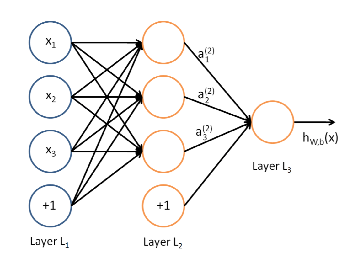
Fig. 2: A simple example of Neural Network.
In this concrete model on the right, we can clearly find out the inputs, weights, biases and outputs.
The first layer is the input layer which includes 2 neurons i_1, i_2 and the bias b_1. The second layer is the hidden layer with 2 neurons h_1, h_2 and the bias b_2. The last layer is the output layer with 2 outputs neurons o_1, o_2. w_i between each layer is the corresponding weight. Here, we assume the sigmoid function is the activation function.
For the convenience of the demonstration on how the backpropagation algorithm actually works, we assign each variable an initial value:
- Input Data: i_1 = 0.05, i_2 = 0.10;
- Output Data: out_1 =0.01,out_2=0.99;
- Initial weights and biases: w_1 = 0.15,w_2=0.20,w_3=0.25,w4=0.30;
w_5 = 0.40, w_6=0.45,w_7=0.50,w_8=0.88;
Out target is: With the input data, the output of the network must approximate to the output data as much as possible.


Step 1 Forward Propagation
Input Layer -----> Hidden Layer:
First, we calculate the weighted input to the h_1 neuron in the hidden layer:z_{h1} = w_1 * i_1 + w_2 * i_2 + b_1 *1 = 0.3775 The output of the h_1 neuron(with the sigmoid activation function) is:
a_{h1} = \frac{1}{1 + e^{- z_{h1} }} = 0.593269992 Similarly, we can get the output of the h_2 neuron is:
a_{h2} = 0.596884378 Hidden Lay ---→ Output Layer:
Repeat the same procedure from above to the output layer:a_{o1} = \frac{1}{1 + e^{- z_{o1} }} = 0.75136507 a_{o2} = \frac{1}{1 + e^{- z_{o2} }} = 0.0.772928465
Here, the forward propagation is finished because we have the output of the network with the input and initial parameters we gave. Apparently, the output value (0.75136079, 0.772928465) differs quite far from the desired output value(0.01,0.99). So,we need to apply the back propagation algorithm to the network to update the parameters and re-calculate output.
Step 2 Back propagation
1. Calculate the error(MSE):
From the first subsection, we knew that:
| E(w,b) = \frac{1}{n} \varSigma_{\vec{x}}||\vec{y}- \vec{f}(\vec{x}) ||^2 |
According to the equation above, we can easily calculate the output of the MSE:
| E(w,b) = E_{o1} + E_{o2} = 0.298371109 |
2. Update the parameters between hidden layer and output layer:
Combine the First equation and the Fourth equation (chain Rule), the derivative of MSE with respect to w_5:
| \frac{\partial E}{\partial w_5} = \frac{\partial E}{\partial a_{o1}}*\frac{\partial a_{o1}}{\partial z_{o1}}*\frac{\partial z_{o1}}{\partial w_5} |

Fig. 5: Back propagate the error for the output layer.(source: 3)
Let's calculate the value of each part from the equation above one by one:
\frac{\partial E}{\partial a_{o1}}:
E(w,b) = \frac{1}{n} \varSigma_{\vec{x}}||\vec{y}- \vec{f}(\vec{x}) ||^2 \frac{\partial E}{\partial a_{o1}} = 2 * \frac{1}{2}*(out_1 - o1 )*(-1) + 0 =0.74136507 \frac{\partial a_{o1}}{\partial z_{o1}}:
a_{o1} = \frac{1}{1 + e^{- z_{o1} }} \frac{\partial a_{o1}}{\partial z_{o1}} = a_{o1}*(1-a_{o1}) = 0.186815602 \frac{\partial z_{o1}}{\partial w_5} :
z_{o1} = w_5 * a_{h1} + w_6*a_{h2} + b_2 *1 \frac{\partial z_{o1}}{\partial w_5} = 1*a_{o1} * w_5^0 +0+0 = 0.593269992
At last, \frac{\partial E}{\partial w_5} =0.082167041.
You may find that we did not use the error variable \delta, then why define it?
Actually we did use it. Relying on the previous equation of \delta, and based on the calculation above, we can easily derive that:
| \frac{\partial z_{o1}}{\partial w_5} = -(out_1-o1) * a_{o1}*(1-o1)*a_{h1} |
Then, \delta can be written as:
| \delta_{o1} = \frac{\partial E}{\partial a_{o1}}*\frac{\partial a_{o1}}{\partial z_{o1}} = \frac{\partial E}{\partial z_{o1}} |
| \delta_{o1} = -(out_1-o1) * a_{o1}*(1-o1) |
So, the derivative of MSE in terms of w_5 is:
| \frac{\partial z_{o1}}{\partial w_5} = \delta_{o1}*a_{h1} |
In this part, the last step is to update the value of w_5 to make our network "better":
| w_5' = w_5 - \eta * \frac{\partial E}{\partial w_5} = 0.35891648 |
where \eta is the learning rate, we take its value as 0.5 here.
Similarly, w_6, w_7,w_8 could be updated to:
| w_6' = 0.408666186 |
| w_7' = 0.511301270 |
| w_8' = 0.561370121 |
3. Update the parameters between hidden layer and input layer:
The method we will use differs not that much from the last part, the only change is: for instance, when we calculate the derivative of total MSE in terms of a_{h1}, the error in both outputs o_1,o_2 should be considered, which means:
| \frac{\partial E}{\partial a_{h1}} = \frac{\partial E_1}{\partial a_{h1}}+\frac{\partial E_2}{\partial a_{h1}} = 0.036350306 |
Based on this, and by the use of Fourth equation \frac{\partial E}{\partial w^l_{jk}} = a^{l-1}_k \delta ^l_j, and Second equation \delta^l = ((w^{l+1})^T \delta^{l+1})\bigodot\sigma'(z^l):
| w_1' = w_1 - \eta * \frac{\partial E}{\partial w_1} = 0.1497870716 |
The same:
| w_2' = 0.19956143 |
| w_3' = 0.24975114 |
| w_4' = 0.29950229 |

Fig. 6: Back propagate the error for the hidden layer.(source:3)
2 Kommentare
Unbekannter Benutzer (ga29mit) sagt:
26. Januar 2017All the comments are SUGGESTIONS and are obviously highly subjective!
Form comments:
Wording comments:
Corrections:
trainingdata consist
training data consists
Widely used method is Mean Squared Errors(MSE)
A widely used method is the Mean Squared Error(MSE)
when x⃗ is input,
when x⃗ is the input,
Besides MSE, cross-entropy error measure is also used in neural networks:
Besides the MSE, the cross-entropy error measure is also used in neural networks:
Batch trainin:
Batch training:
Recapping, our goal
To recap, our goal
Now, of course, for the function plotted above, we can eyeball the graph
Now, for the function plotted above, we can examine the graph
But actually we do not know where is the exact point at which E(θ1,θ2) reaches its minimum
But actually, we do not know at which point exactly E(θ1,θ2) reaches its minimum
where η is the learning rate which is a small, positive parameter.
where η is the learning rate (a small, positive parameter).
Then from cost equation we are clear that
Thereby, we can infer from the cost equation that
In Newton's Method, due to the use of second-order information of the cost function, the algorithm performs faster convergence.
Due to the use of second-order information of the cost function in Newton's Method, the algorithm shows a faster convergence.
The main drawback of this method is computationally expensive for evaluation and inversion
The main drawback of this method is its computational expensiveness for evaluation and inversion
But firstly we should make it clear: could the parameters all be initialized to zero?
But first we should clarify if the parameters can all be initialized to zero?
In above, we discussed
In the previous section, we discussed
How to optimize each parameter in a multi-layered neural networks
How should each parameter in a multi-layered neural network be optimized?
Firstly, assume the weighted input to the jth neuron in layer l:
First, assume the weighted input to the jth neuron in layer l equals:
output of k-th neuron
output of the k-th neuron
Now, let's see in a neural network how these 4 equations could be used.
Now, let us see how these 4 equations could be used in a neural network.
This is just a brief view of neural network which means, it is not enough
This is just a brief view of neural network, which means it is not enough
In this concret model on the right
In this concrete model on the right
Here, we assume sigmoid function is the activation function.
Here, we assume the sigmoid function as the activation function.
For the convenience of demonstration how the backpropagation algorithm actually works,
For the convenience of the demonstration on how the backpropagation algorithm actually works,
First we calculate the weighted input to the h1 neuron in hidden layer:
First, we calculate the weighted input to the h1 neuron in the hidden layer:
output of the h2 neuron is:
output of the h2 neuron which is
and re-calculate output.
and re-calculate the output.
we know that:
we knew that:
output of the MES:
output of the MSE:
You may found that, we didn't use
You may find that we did not use
Rely on the previous equation of δ, and
Relying on the previous equation of δ and
learning rate, we take its value as 0.5 here.
learning rate (here arbitrarily chosen to be 0.5)
much from last part,
much from the last part,
The next, we need to do it recursively until the error converges or the number of iteration reached the limitation.
As a net step, we need to apply it recursively until the error converges or the number of iteration reached a set limit.
a satisfied performance.
a satisfactory performance.
Confusion:
Individual fully connected layers function identically (???) to the layers of the multilayer perceptron with the only exception being the input layer. (a verb is missing here)
Final remark:
Unbekannter Benutzer (ga58zak) sagt:
28. Januar 2017Hello,
Form comments:
Confusion:
When you talk about the optimization methods, there are Gradient descent, Stochastic gradient descent, momentum, adam and so on, these are optimization methods.
But Backpropagation is the way you update your weights and biases based on a given optimization methods. Backpropagation does not belong to a optimization method, this is my understanding.
You directly mention the optimization in subsection Error Backpropagation and do not mention Gradient descent, that is my confusion.
Suggested change and some errors: