Christoph Fraundorfer, winter semester 2018/19
Machine learning is the most prominent part of Artificial Intelligence (AI) in today's time. Its most common methods are based on neural networks, which can be used to find unknown solutions to problems and for optimization. In the past few years many methods were developed in the area of image and natural language processing, which can also be applied in other areas, for example in non destructive testing (NDT).
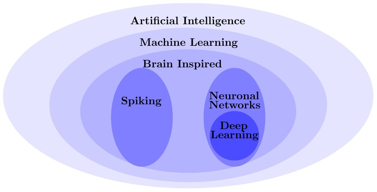
| The figure describes the classification of machine learning in the field of AI, as well as its underlying concepts [1]. |
Machine Learning as Part of Artificial Intelligence
The term "AI" itself was defined in the 1950s by John McCarthy [1]. Advances in research strive to develop an "Artificial General Intelligence", which is able to solve general problems like the human mind [2]. Machine learning itslef on the other hand was coined by Arthur Samuel in the later 1950s as an algorithm, which is able to learn connections, which are not concretely described in its code [1]. Motivations to implement such an algorithm were mostly found in the biology of the brain. This is the reason why the first methods describing the principles of learning were already formulated in the 1940s by Donald Hebb [3], Warren McCulloch and Walter Pitts [4]. The latter assumed, that each neuron in the brain was binary and had a finite threshold [5]. Based on this theory the concept of artificial neural networks (ANN) was developed and became the foundation of most of the research in the area of machine learning. Other advances were made with approaches in spiking, which is also inspired by the brain and lays its focus on the impulse function responsible for activating neurons [1]. The trend of application, however, is moving towards neural networks in the form of deep learning, which emphasizes the repeatedly and intertwined use of the concept [6] in the form of a multiple layered structure, like in the human brain. The categorization of the introduced terms is visualized in figure "Classification of Machine Learning in AI".
Machine Learning Today
As already mentioned, McCulloch and Pitts laid the theoretical foundation on the structure of how a neural network can be implemented. Also already part of their theory was that a network could be constructed with multiple synapses between these nodes. After Hebb added the knowledge that memory is stored in the connections, Frank Rosenblatt introduced the adjusting of variable weights in the node as concept for storing information in the 1960s. He also provided the mathematical conditions of existence for solutions and proofed the convergence of algorithms using these concepts. In the 1980s researchers achieved further developments, but also understood that machine learning was mainly limited by the provision of data and computational power [[5], [1]]. Since computational power has increased immensely in the form of graphical processing units (GPUs) or tensor processing units (TPUs) in the last 30 years and large amounts of labeled data have been created, these limitations have been overcome and machine learning with neural networks is again on the advance. Today any ANN is connected over a collection of neurons, which can be separated into the three parts input layer, at least one hidden layer and an output layer. In order to learn, the algorithm has to be provided with a lot of data. The nodes of the neurons in the hidden and output layer are then connected by simple linear combinations of x_i neuron connections including their weights w_{ij} described by
\hat{y}_j = \sigma(a_{j}) = \sigma \left( \sum_{i=1}^{D} w_{ij}x_{i} + w_{0} \right) \quad \quad \quad \quad \quad \quad (1)
where w_0 is a bias, which can be chosen. a_j is known as the activation and is inserted in a differentiable, nonlinear activation function \sigma, often a sigmoid function, which generates the value \hat{y}_j for the linear combination of the next layer. This type of formular can be propagated through the whole network until the output layer, which consists of at least one node and specifies whether a binary question is true or not. This forward-propagating is depicted in figure "Forward-propagation in a Neural Network". Depending on the correctness of this value the algorithm can be trained and weights and biases changed via backpropagation until the desired result is achieved in the case of supervised learning. After the training the neural network can be tested and used on new data to provide answers according to the learned mapping [7]. Weights and biases can be chosen randomly in the beginning of the procedure. Finally, the chance and dificulty of this method of providing a correct neural network is the number of layers and nodes used inside them, as well as the form of the activation function, which can both be specified by the user. Typical ANN applications are finding and optimizing non-linear connections and forecasting. Other uses are for example image processing, where convolutional neural networks (CNN) are trained to identify certain structures in pictures, or language processing, where recurrent neural networks (RNN) can store information dependent on time.
| The figure describes the forward-propagation in a multilayer perceptron (MLP). Red numbers indicate the linear combination of the black numbers, which are the initial random weights and biases. Inserting these into an activation function, which is defined by the user, a sigmoid function in this case, results in the blue numbers as weights of the nodes. In the end the question is, whether according nodes in the output layer should be 0 or 1. Depending on this the neural network can be trained via back-propagation. |
Theoretical Background of Neural Networks
Machine Learning Taxonomy
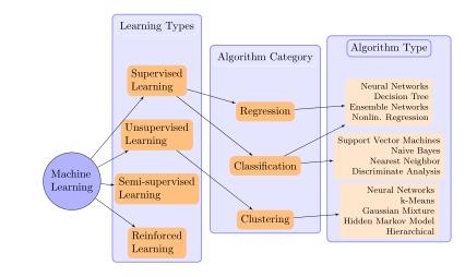
When input and output data is given in pairs, i.e. there are labeled inputs according to the output data values, the approach is called supervised. In this case it is easy to provide information from which the system can learn the input to output mapping. If the input vectors can be assigned to discrete values the problem is called classification problem. If, on the other hand, the output consists of one or more continuous variables, the problem is called regression problem. In an unsupervised problem no pairs are given and the system itself discovers patterns in the data during training. Methods used in this category rely on similar output of the system according to the input, they are therefore able to identify commonalities and relate them to the specific inputs. A typical example is clustering [7]. In the semi-supervised learning, where the input data is incomplete or noisy, the representative is called active learning, which queries for another similar output for a new input. Since many methods are able to sort unknown data according to the input, the system can profit from only partially labeled data, if it has only a few reference points. In case of a dynamic environment reinforced learning is applied, which improves its behavior by checking the response from it. Methods of this category aim not for accuracy but for performance by balancing new information with already known data. These classifications and suggested methods to solve the respective problems are depicted in Figure 3.
| The figure describes the classification of diferent methods in machine learning. Note that the method, which can solve all problem types is the neural network. |
Gradient Descent
As already mentioned above, the forward- and back-propagation is the underlying principle of the training algorithm. It maps input data to labeled output data. In figure "Forward-propagation in a Neural Network" it is also indicated, values are propagated to the end neuron to a final value \hat{y} by repeatedly calculating equation 1 for each neuron until the output layer is reached. After this forward propagation is calculated with random weights and biases, the output value will differ from the expected result. To get the measure of this error, loss functions are used, where the most common is the sum-of-squares or L_2 error, which is defined as the squared difference between the desired value y_j and the propagated value \hat{y}_j:
L_{2} = \frac{1}{2}\left(\hat{y}_{j}-y_{j}\right)^2 \quad \quad \quad \quad \quad \quad (2)
In the process of back-propagation the loss function can be used to adjust the weights and biases by using its derivative. Increasing or reducing the values according to the desired value can be evaluated with gradient descent or similar methods, like for example conjugate gradient. Calculating the derivative of the error for one single neuron implies the double application of the chain rule, yielding
\frac{\partial L_2}{\partial w_{ij}}= \frac{\partial L_2}{\partial \hat{y}_{j}} \cdot \frac{\partial \hat{y}_{j}}{\partial a_{j}} \cdot \frac{\partial a_{j}}{\partial w_{ij}} \quad \quad \quad \quad \quad \quad (3)
where a_j is the value of the node linear combination, y_j is the desired value, w_{ij} are again the weights and \hat{y}_j is the output of neuron j and calculated with equation (1). Calculating each component respectively in order to evaluate equation (3) yields
\frac{\partial L_2}{\partial \hat{y_{j}}} = (\hat{y}_{j}-y_{j}), \quad \frac{\partial \hat{y}_{j}}{\partial a_{j}} = \sigma'(a_{j}), \quad \frac{\partial a_{j}}{\partial w_{ij}} = \sum_{i=1}^{D}x_{i}\quad \quad \quad \quad \quad \quad (4)
and finally:
\frac{\partial L_2}{\partial w_{ij}} = (\hat{y}_{j}-y_{j})\cdot \sigma'(a_{j}) \cdot \sum_{i=1}^{D}x_{i} \quad \quad \quad \quad \quad \quad (5)
This simple example is just one part of the whole gradient vector, which is built from the derivative of the cost or loss function w.r.t. the weights and biases. This idea can then be expanded to more layers and more neurons per layer by including more indices. Finally, it can be concluded, that these chain rule expressions give the derivative, which determine each component of the gradient, needed for propagating the error to the weights [[7], [8]]. After that the weights are adjusted according to this error with:
w_{ij}^{new} = w_{ij}^{old} + \Delta w_{ij}\quad \quad \quad \quad \quad \quad (6)
Overfitting
The essence of the algorithm is to assimilate the input-output mapping by adjusting the weights and threshold functions accordingly or in other words to learn from the past to predict the future. If the training is not sufficient enough the neural network is not able to map reliably between the input data and output afterwards. If, however, the algorithm learns too many input-output examples, it can end up memorizing the data. This is called overfitting. Such an overfitting makes the network inefficient because it is not able to recognize slightly different data anymore [8]. It occurs in general when the network is too complex relative to the noisiness of the training data. One way to illustrate over- and underfitting is displayed in figure "Over- and Underfitting of Data Points". Regularization can help to avoid the false representation of data points, which is the instruction of either constraining the degrees of freedom in the case of overfitting or adding them in the case of underfitting. Typical methods using this principle are for example linear regression, ridge regression [9] or lasso regression [10].
| The figure shows how data points are fitted with a function. While a linear function underfits (left) the data, a high polynomial function overfits (right) the points. Both of them fail to represent the data distribution, however a low polynomial function (middle) is a good fit in this case. |
Evaluation of the Network
Typical Approach
In general the processing of data via neural networks can be performed with the following main steps [10].
- Look at the big picture.
- Get the data.
- Discover and visualize the data to gain insights.
- Prepare the data for machine learning algorithms.
- Select a model and train it.
- Fine-tune your model.
- Present your solution.
- Launch, monitor, and maintain your system.
Common Evaluation Methods
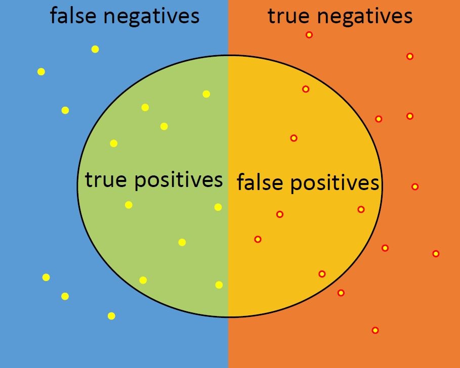
There are several methods to measure the performance of a classification problem, for example via precision and recall or with a confusion matrix [10]. The latter is constructed by counting the number of wrong predictions in a single iteration of cross validation, where the test data is still unknown to the trained model. When counting, the result can be displayed in a matrix using the actual class of the data as column and the eventually wrong predicted class as row, as is shown in figure "Illustration of a Confusion Matrix". Looking at the confusion matrix in the end allows to qualify the performance, where a perfect classifier only has true positives and true negatives and none false negatives or false positives, meaning only main diagonal entries. If an even preciser performance measurement for the classification problem is needed, precision and recall, which are based on the results of the confusion matrix and can be illustrated similar to figure "Another Interpretation of the Confusion Matrix", can be used. While precision is measured as the quotient of true positive and the sum of false positive and true positive classifications, recall uses the quotient of true positive and the sum of false negative and true positive classifications.
\mbox{precision} = \frac{TP}{TP + FP} \quad \quad \mbox{recall} = \frac{TP}{TP + FN}\quad \quad \quad \quad \quad \quad (7)
Using a combination of them can help to estimate the accuracy of the predictions, where precision is the equivalent to correctness and recall can be interpreted as sensitivity of the system. Unfortunately it is not always possible to keep both values high because of the precision/recall trade off [10].
| Exemplary distribution of predicting rivets' head height with a neural network. The distribution among the equally named rows, represent the predictions of the network. With an optimally performing network, the red cells contain only zero (no wrong classification) and the green cells the total number of each category (all instanced of each category were predicted correctly). | This illustration depicts the correctly and incorrectly classified samples of a training algorithm. The four areas categorize true positives (TP), true negatives (TN), false positives (FP) and false negatives (FN). Note that in a correct classification all samples in the blue area should result in the green category. |
How to Improve the Network's Performance
There is a good chance, that a model in machine learning has an unsatisfactory performance, however, this performance can be improved by simple strategies. One of the most effective ones is the already mentioned cross validation, where the training, validation and test data is interchanged in several iterations and overfitting of the network is reduced. In order to avoid over- and underfitting and to get a good generalization this method divides the available data into parts of which one major part is used for training, one part for validation of the learning process and the last part for testing. By interchanging these parts in subsequent iterations a better performance and capturing especially abnormal data can be achieved [8]. Another method in order to improve the performance is \textbf{batch normalization}. It addresses the problem, that the distribution of each layer’s input values changes during training, as the parameters of the previous layers change. The technique adds an operation before the activation function of each layer, which evaluates the mean and standard deviation of the current inputs. After zero-centering and normalizing the batches with theses values an improvement of the network can be observed [10]. Another common method are Ensemble methods. A combination of models can perform better than the best individual model, especially if different error types are involved. Typical techniques are for example boosting and bagging. The first relies on training a predictor that tries to correct its predecessor by sequentially focusing more on underfitted data. The latter creates a new predictor by training them on a random subset of the training set [10].
Additionally to these approaches any network can be improved by adding more data. More data leads to more cases, which can be considered, and cause more generalization and therefore an overall improvement of the model. Obviously such data has to be available, which is sometimes not the case.
Finally, feature engineering in general can also improve a network's performance. By thoroughly analyzing the data and using expert knowledge on it, it is possible to describe a lot of the variability of the data in advance and cause a reduction of variables in the system. It is very important to include correlations in a preprocessing step to increase the performance. Additionally to this, also while working with the data further features can be both found and included, which also will cause an improvement of the network [7].
Finally, another method of sampling is the stratified sampling. In this procedure the subpopulation of a batch is chosen according to the distribution of the subpopulation in the whole set. With this the bias of the single batches can be adjusted to the actual sample distribution, while variance is reduced [10].
Machine Learning in NDT Applications
In general, non-destructive testing (NDT) applications rely on acquiring information from the interaction between a specimen and material- or electromagnetic waves. Examples are:
- Ultrasound
- X-Ray
- Non-ionizing Radiation
- Infrared Thermography
- Radio Detection and Ranging (RADAR) Testing
- Microwave Testing
- Material Waves
- Other Visualization Techniques
This information has to be treated accordingly and visualized [11] to make assessments about the materials and structures, which are investigated. Machine learning has the potential to provide assistance in detecting and interpreting signals arising from these testing methods and can improve the results as well as optimize the evaluation processes. Examples of the application of neural networks in NDT:
- Detecting pore space in CT soil images: A deeper analysis of the areas, where pore and soil are mixed could be performed and 96 \% of the pore spaces could be classified correctly [12].
- Estimating the ethanol concentration in beverages through vibrational spectroscopy without opening them [13].
- Detecting the position of failures in a FEM model of a concrete pillar investigated with ultrasound technique [14]
- Detecting of failures in composite structures [15]
- Classification of rivet joints in CT data [16]
Especially the last examples indicate, how neuronal networks can favor NDT in structured and well defined, as well as in unstructured material.
Easy Access Tools
Easy access to the functionality of neuronal networks is provided by Google Playgorund https://playground.tensorflow.org/, where different sets of data points can be trained. For even better understanding it is recommended to implement a simple machine learning algorithm according to one of the many guidelines and tutorials provided by the internet or books to this topic, for example in Python https://www.anaconda.com/download/ or with https://github.com/ageron/handson-ml.
Literature
- Christopher M. Bishop. Pattern recognition and machine learning. Information science and statistics. Springer, New York, NY, corrected at 8th printing 2009 edition, 2009. ISBN-10: 0-387-31073-8 ISBN-13: 978-0387-31073-2
- James M. Keller, Derong Liu, and David B. Fogel. Fundamentals of computational intelligence: Neural networks, fuzzy systems, and evolutionary computation. IEEE Press series on computational intelligence. IEEE Press Wiley and IEEE Xplore, Hoboken, New Jersey and Piscataway, New Jersey, 2016. ISBN: 978-1-110-21434-2
- Aurèlien Gèron. Hands-on machine learning with Scikit-Learn and TensorFlow: Concepts, tools, and techniques to build intelligent systems.O'Reilly Media, Sebastopol, CA, first edition edition, 2017. ISBN: 978-1-491-96229-9
References
- Vivienne Sze, Yu-Hsin Chen, Tien-Ju Yang, and Joel S. Emer. Efficient processing of deep neural networks: A tutorial and survey. Proceedings of the IEEE, 105(12):2295-2329, 2017.
- Matthew Iklfie, Arthur Franz, Rafal Rzepka, and Ben Goertzel. Artificial General Intelligence, volume 10999. Springer International Publishing, Cham, 2018.
- Donald Olding Hebb. The organization of behavior: A neuropsychological theory. L. Erlbaum Associates, Mahwah, N.J, 2002.
- Warren S. McCulloch andWalter Pitts: A logical calculus of the ideas immanent in nervous activity. Bulletin of Mathematical Biophysics, 5(4):115-133, 1943.
- J. B. Pollack. Connectionism: past, present, and future. Artificial Intelligence Review, 3(1):3-20, 1989.
- Boris Kryzhanovsky, Witali Dunin-Barkowski, and Vladimir Redko. Advances in Neural Computation, Machine Learning, and Cognitive Research, volume 736. Springer International Publishing, Cham, 2018.
- Christopher M. Bishop. Pattern recognition and machine learning. Information science and statistics. Springer, New York, NY, corrected at 8th printing 2009 edition, 2009.
- James M. Keller, Derong Liu, and David B. Fogel. Fundamentals of computational intelligence: Neural networks, fuzzy systems, and evolutionary computation. IEEE Press series on computational intelligence. IEEE Press Wiley and IEEE Xplore, Hoboken, New Jersey and Piscataway, New Jersey, 2016.
- Shubaham Jain. A comprehensive beginners guide for linear, ridge and lasso regression,[1] 22.06.2017.
- Aurèlien Gèron. Hands-on machine learning with Scikit-Learn and TensorFlow: Concepts, tools, and techniques to build intelligent systems.O'Reilly Media, Sebastopol, CA, first edition edition, 2017.
- Fernando Puente León and Uwe Kiencke. Messtechnik.Springer Berlin Heidelberg, Berlin, Heidelberg, 2011.
- M. G. Cortina-Januchs, J. Quintanilla-Dominguez, A. Vega-Corona, A. M. Tarquis, and D. Andina. Detection of pore space in ct soil images using artificial neural networks.Biogeosciences, 8(2):279-288, 2011.
- James Large, E. Kate Kemsley, Nikolaus Wellner, Ian Goodall, and Anthony Bagnall. Detecting forged alcohol non-invasively through vibrational spectroscopy and machine learning. In Dinh Phung, Vincent S. Tseng, Geoffrey I. Webb, Bao Ho, Mohadeseh Ganji, and Lida Rashidi, editors, Advances in Knowledge Discovery and Data Mining, volume 10937 of Lecture Notes in Computer Science, pages 298-309. Springer International Publishing, Cham, 2018.
- Osvaldo Gervasi, Beniamino Murgante, Antonio Laganfia, David Taniar, Youngsong Mun, and Marina L. Gavrilova, editors. Computational Science and Its Applications - ICCSA 2008. Lecture Notes in Computer Science. Springer Berlin Heidelberg, Berlin, Heidelberg, 2008.
- Jonas Holtmann. Neural Networks in Non-Destructive Testing. TUM, 2018.
- Fabian Diewald. Autonomous Classification of Rivet Joints Based on Computed Tomography Data. TUM, 2018.


