Artificial Neural Networks

Introduction to Neural Networks

In computer science, artificial neural networks, also referred to as ANNs, are a computational information processing approach inspired by the mammalian nervous system. ANNs consist of a large number of interconnected elementary processing units called artificial neurons, whose structure and functionality are modeled after the biological neurons.⁽¹⁾

In comparison to conventional problem solving methods, artificial neural networks offer an adaptive approach to solve various problems through their ability to learn. Conventional algorithms usually focus on solving specific problems using a set of instructions. Therefore in order to solve a problem using these systems, a certain solution needs to be known and implemented.

In contrast, artificial neural networks do not rely on a complex processing system but a number of interconnected neurons, which operate in parallel according to the input given. While they are not constructed to solve a specific problem, they can be trained by using a set of examples. Throughout this learning process the network adjusts and adapts itself similar to the human learning process.

Inspiration

In biology, a nervous system consists of a number of specialized cells called neurons that communicate with each other through a number of complex connections. These cells have the ability to transmit information utilizing electrical and chemical signals and this communication process is called neurotransmission.

In a nervous system, this connectivity between neurons creates a structure called a neural network in which a neuron is linked to other neurons by its dendrites. These dendrites serve as a receptor and listen to incoming signals from other neurons. Depending on this input signal, the cell body may send an impulse through its axon to transmit a new signal to other neurons using the axon terminals, which are received by dendrites of other neurons.

The structure of an artificial neuron, illustrated in figure 2, was based on this concept⁽²⁾. Similar to a biological neuron, a simple processing unit receives a signal and generates an output depending on the input.

In more detail, this process is carried out in 4 steps:

Receiving information: the processing unit obtains the information as input $\begin{array}{l}x_1, x_2,...., x_n\end{array}$ .
Weighting: each input is weighted by its corresponding weights denoted as $\begin{array}{l}w_0, w_1, w_2, ...., w_n\end{array}$ .
Activation: an activation function $\begin{array}{l}f\end{array}$ is applied to the sum of all the weighted inputs $\begin{array}{l}z\end{array}$ .
Output: an output is $\begin{array}{l}y\end{array}$ generated depending on $\begin{array}{l}z\end{array}$ .

$\begin{array}{l}\displaystyle y = f(z) \quad \text{where} \quad z = \sum_{i=1}^n w_i x_i + w_0\end{array}$

The Structure of Neural Networks

Neural networks consist of a number interconnected neurons. Depending on their inputs and outputs, these neurons are generally arranged into three different layers as illustrated in figure 3.

Input Layer: The input layer is the first layer in an artificial neural network and it is dimensioned according to the input. It serves as an interface between the data and the network.
Hidden Layer(s): The hidden layer(s) consist of a number of connected neurons, which allow the information to be processed and transmitted from the input layer, between hidden layers and ultimately to the output layer.
Output Layer: The output layer is the last layer in the network and similar to the input layer it is dimensioned to fit the proper output. It represents the result of the information process.

Depending on the connectivity between the neurons in the hidden layer, the type of the neural network can be divided into two categories, namely Feed-Forward and Feedback Networks.

Feed-Forward Networks

In a feed-forward neural network, the information only flows in one direction, from input to output. The output of each neuron in the hidden layer is passed to another neuron as an input in the next layer. Since there are no possible loops within the structure, the information process is finished once it reaches the output layer.

Feedback Networks

In a feedback network, the information can travel in both directions, which means a neuron can be linked to any neuron within the hidden layer regardless of the layer hierarchy. This structure allows the network to have loops, where the information can flow continuously and update the network until it reaches a state of equilibrium.

Applications

The learning capabilities of artificial neural networks along with their flexibility make them an attractive approach for many tasks. Nowadays, they are used in a wide spectrum of areas including but not limited to Pattern Recognition, Classification, Function Approximation and Regression, Signal Processing, Time Series Estimation.

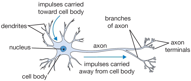
Figure 1: the structure of a basic biological neuron⁽⁶⁾

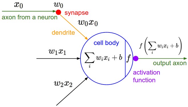
Figure 2: the structure of a single artificial neuron⁽⁶⁾

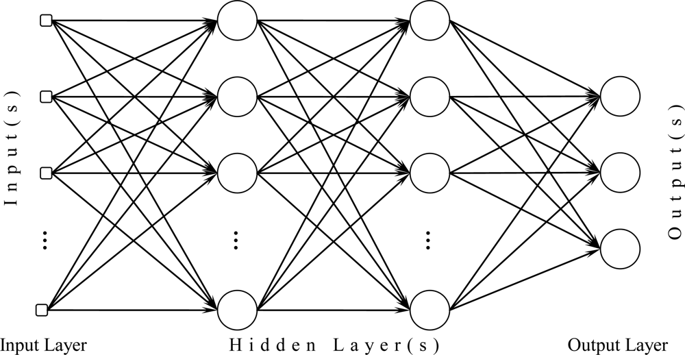
Figure 3: the structure of a fully connected 3-Layer neural network (image source)

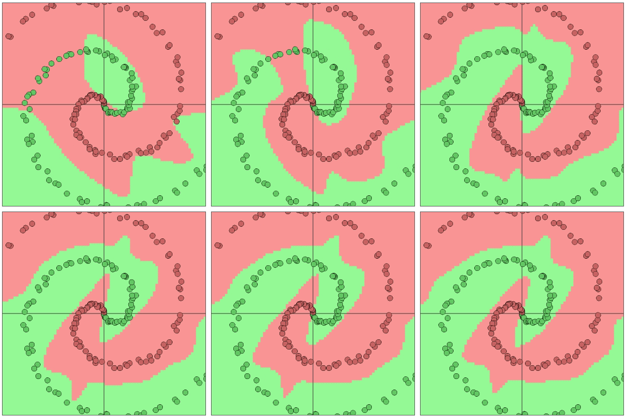
Figure 4: the illustration of a neural network solving a two dimensional classification problem with two distinguishable classes ⁽⁷⁾

Multilayer Perceptrons

A multilayer perceptron, also referred to as MLP, is a feed-forward artificial neural network and it consist of multiple layers, which are fully connected to each other. In other words, every single neuron in a multilayer perceptron is linked to the neurons in the next layer.

Figure 5 demonstrates the general structure of a $\begin{array}{l}(L+1)\end{array}$ -Layer perceptron which consists of one input layer, $\begin{array}{l}L\end{array}$ hidden layers and one output layer. The number of neurons in the input layers is denoted by $\begin{array}{l}D\end{array}$ and the number of neurons in the output layer is denoted by $\begin{array}{l}C\end{array}$ . Using this notation the output of the $\begin{array}{l}i\end{array}$ th neuron in $\begin{array}{l}l\end{array}$ th layer can be computed as:

$\begin{array}{l}\displaystyle y_i^l = f(z_i^l) \quad \text{where} \quad z_i^l = \sum_{k=1}^{m^{(l-1)}} w_{i,k}^{l} y_k^{l-1} + w_{i,0}^l\end{array}$

where the $\begin{array}{l}m_l\end{array}$ denotes the number of neurons in the $\begin{array}{l}l\end{array}$ th hidden layer. The activation function is denoted by $\begin{array}{l}f\end{array}$ and weights are represented as $\begin{array}{l}w\end{array}$ where $\begin{array}{l}w_{i,k}^l\end{array}$ is the weight from the $\begin{array}{l}k\end{array}$ th neuron in $\begin{array}{l}(l-1)\end{array}$ th layer to the $\begin{array}{l}i\end{array}$ th neuron in the $\begin{array}{l}l\end{array}$ th layer. $\begin{array}{l}w_{i,0}^l\end{array}$ serves as the external input called the bias for the $\begin{array}{l}i\end{array}$ th unit in $\begin{array}{l}l\end{array}$ th layer.⁽⁴⁾

In a more compact form, the functionality of a multilayer perceptron, which maps $\begin{array}{l}D\end{array}$ inputs into $\begin{array}{l}C\end{array}$ outputs, can be formulated as⁽³⁾:

$\begin{array}{l}\displaystyle y(.,w): \mathbb{R}^D \to \mathbb{R}^C, x \mapsto y(x,w)\end{array}$

The training of these networks is considered to be a challenging task, especially in deep neural networks. They require proper fine-tuning and initilization and must be designed carefully.

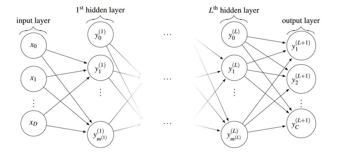
Figure 5: the illustration of a fully connected $\begin{array}{l}(L+1)\end{array}$ -layer perceptron with $\begin{array}{l}D\end{array}$ inputs and $\begin{array}{l}C\end{array}$ output neurons ⁽³⁾

Activation Functions

The activation function F of a neuron represents the function which maps its weighted inputs into an output and as a result determines its behavior.

$\begin{array}{l}\displaystyle y = f(z) \quad \text{where} \quad z = \sum_{i=1}^n w_i x_i + w_0\end{array}$

There are many different forms of possible activation functions for neural networks and this section covers some of the most preferred ones briefly introducing their advantages and disadvantages.

Threshold Function

A threshold function is a function which generates the output $\begin{array}{l}1\end{array}$ if the input exceeds a certain value $\begin{array}{l}n\end{array}$ . If this criteria is not fulfilled, this function takes the value $\begin{array}{l}0\end{array}$ .

A common threshold function is the Heaviside step function ( $\begin{array}{l}n=0\end{array}$ ) which can be defined as:

$\begin{array}{l}H(x) = \begin{cases} 0 & \text{if } x< 0\\ 1 & \text{if } x\geq 0\ \end{cases}\end{array}$

This function does not offer a good solution since it does not fulfill the requirements of the backpropagation process of a neuron.

Sigmoid Function

The sigmoid function is one of the most widely used activation functions and brings a solution to the problem mentioned above. It generates an S-shaped curve, which maps its inputs into the interval of values of $\begin{array}{l}]0,1[\end{array}$ . The sigmoid function has a non-zero gradient throughout its definition region, which makes it a good candidate when utilizing the backpropagation algorithm.

$\begin{array}{l}\displaystyle \sigma(x) = \dfrac{1}{1+e^{-x}}\end{array}$

On the other hand, using a sigmoid function has its own drawbacks. One of the main problems encountered while using a sigmoid activation function is called the vanishing gradient problem. At each step of backpropagation, the weights are updated according to the gradient of the error function with respect to the weights. If the neuron gets saturated, the gradient can become significantly small, preventing a successful training process.

It is also important to note, that the output values of a sigmoid function are not zero centered. As a result, the gradient values at each step of the backpropagation process can only be all negative or all positive depending on the gradient of the error. This problem can decelerate the training process of a neural network.

Hyperbolic Tangent Function

Similar to the sigmoid function, a hyperbolic tangent function (a $\begin{array}{l}tanh\end{array}$ function) generates a S-shaped curve but it maps its inputs to values $\begin{array}{l}]-1,1[\end{array}$ . Even though, a $\begin{array}{l}tanh\end{array}$ neuron still suffers from the vanishing gradient problem, it generates zero-centered outputs and eliminates the problem mentioned above.

$\begin{array}{l}\displaystyle f(x) = tanh(x)\end{array}$

Rectified Linear Units

The rectified linear units, also referred to as ReLUs, utilize a specialized ramp function for the activation, which is formulated as:

$\begin{array}{l}\displaystyle f(x) = max(0,x)\end{array}$

Since they use a computationally less complex ramp function for the activation, these units are considered as an useful alternative to the sigmoid and $\begin{array}{l}tanh\end{array}$ function, particularly in more complex structures featuring millions of neurons (such as convolutional neural networks⁽⁵⁾). More detail about the advantages of rectified linear units in these structures can be found in section "Layers of a convolutional neural network".