10: Goal-specific brain MRI harmonization

Lijun An, Jianzhong Chen, Pansheng Chen, Chen Zhang , Tong He, Christopher Chen, Juan Helen Zhou, B.T. Thomas Yeo

Blog post written by: Unbekannter Benutzer (ge32zix) 

1. Introduction

Magnetic Resonance Imaging (MRI) is a functional and morphological imaging technique widely used in clinical studies. MRI offers high flexibility in imaging, for example, we can acquire T1-weighted or T2-weighted images by changing the repetition time (TR) and echo time (TE). This flexibility allows us to achieve different contrasts in different cases but also introduces significant variability across different MRI datasets. These variations may come from:

• hardware: magnetic field strength, scanner manufacturer, receiver coil hardware, etc.
• reconstruction algorithms
• acquisition parameters: voxel size, echo time, etc.
• variations from patients: age, sex, race, diagnosis, etc.

For example, Figure 1 shows us an example of how acquisition parameters make a difference in MRI scans:

Figure 1: T1-weighted MRI images with different acquisition parameters [1]

These variations can sometimes be undesirable. Imagine, we want to build a neural network to predict Alzheimer's disease so we want as much MRI data as possible. But due to dataset variations, two healthy scans from distinct datasets may look more different than a healthy scan compared to a diseased scan from the same dataset. In this case, the amount of data that we can use is limited, which may consequently limit the generalizability or reproducibility of our model.

Fortunately, there is a technique named MRI harmonization, which aims to remove unwanted MRI dataset differences. Based on this, we can potentially boost statistical power and build models that generalize better.

2. Related Work

MRI harmonization methods can be divided into two broad categories: statistical models and image-level models. Statistical models focus on regional volumes (e.g. ROIs) of images and perform post-processing harmonization. Representative methods are ComBat [2] and its variants. For image-level models, the input and output are both images, and they can be further divided into paired mapping models and unpaired mapping models. Paired mapping models require paired data, which means that the same brains should be scanned at all sites. However, this is expensive and time-consuming. To avoid reliance on paired data, unpaired mapping methods are proposed, such as Cycle-Consistent Adversarial Network [3] and Variational Autoencoder (VAE) [4], as shown in Figure 2.

Figure 2: MRI harmonization models

But there is a common drawback of all the previous methods: they don't consider downstream tasks. However, unwanted dataset differences can vary according to different downstream applications. Let's consider two cases:

1. We'd like to develop an Alzheimer’s disease (AD) prediction model that is generalizable across different racial groups, then race might be considered as an undesirable dataset difference

2. We'd like to predict AD progression in different racial groups, then race needs to be preserved

Therefore, overlooking downstream applications may potentially limit downstream performance. Aiming to tackle this, the authors of this paper design a goal-specific harmonization model, which is compared to two baseline harmonization models: ComBat and cVAE. More details are shown in the next section.

3. Methods

3.1 Datasets and Preprocessing

In this paper, T1 structural MRI data from three datasets are considered: Alzheimer’s Disease Neuroimaging Initiative (ADNI), Australian Imaging, Biomarkers and Lifestyle (AIBL), and Singapore Memory Ageing and Cognition center (MACC). It is assumed that there is no site difference in one single dataset. Harmonization is performed with volumes of regions of interest (ROIs) across datasets, before which cortical and subcortical ROIs are defined based on the FreeSurfer software [6]. 

This paper studies the harmonization between AIBL and ADNI, as well as MACC and ADNI. For simplicity, in this chapter, only the harmonization process between AIBL and ADNI is shown, and the same process is also performed for MACC and ADNI.

3.2 Baseline Harmonization Models

ComBat [2]

ComBat is a linear mixed effects model that tries to eliminate additive and multiplicative site effects:

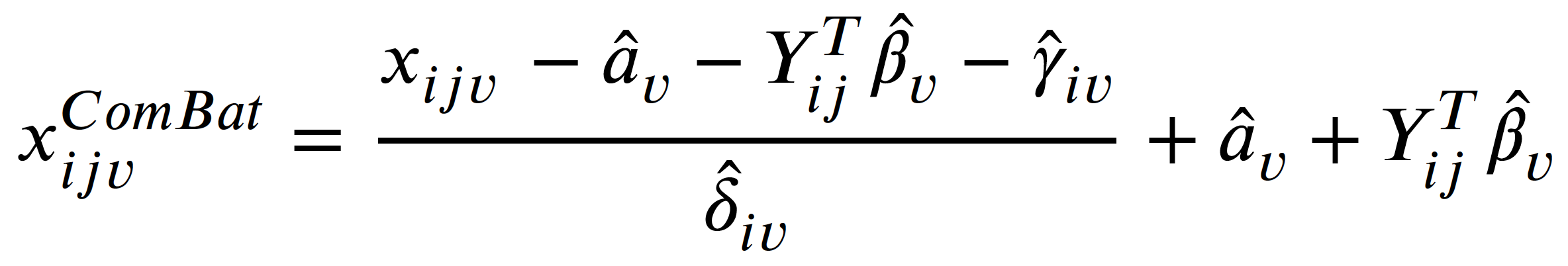
where:

• 𝑥_𝑖𝑗𝑣 is the volume of the 𝑣-th brain ROI of subject 𝑗 from site 𝑖
• 𝛼_𝑣 is the average measure for the reference site
• 𝑌_𝑖𝑗 is covariate of subject 𝑗 from site 𝑖
• 𝛽_𝑣 is the coefficient of 𝑌
• 𝛾_𝑖𝑣 is an additive site effect
• 𝛿_𝑖𝑣 is a multiplicative site effect
• 𝜀_𝑖𝑗𝑣 is the residual error term following a normal distribution with zero mean
• A parameter with ^ means it is estimated from the data

Figure 3: Some sample ROIs in the image are displayed in different colors.

However, ComBat considers brain regions (i.e. ROIs) separately, as shown in Figure 3, hence may not be able to remove site differences that are across regions.

cVAE [4]

Conditional VAE is a variant of VAE, and the architecture is shown in Figure 4. Compared to a normal VAE, it adds a condition to control for output and a discriminator to further make output similar to the input. 

Figure 4: Architecture of cVAE with items of its loss function

The encoder maps data x to a representation z that is independent of s, where s is the site information. Further, this representation is concatenated with s, and input into the decoder to reconstruct x.

In implementation, Both the encoder and the decoder are fully-connected networks, and s is a one-hot encoder. The loss function of cVAE is:

where:

• L_recon is the reconstruction error, i.e. mean square error (MSE)
• L_prior is the Kullback–Leibler divergence between representation z and Gaussian distribution
• L_adv is the cross-entropy loss of an adversarial discriminator seeking to distinguish between $//<![CDATA[ \begin{array}{l}x\end{array} //]]>$ and $//<![CDATA[ \begin{array}{l}\hat{x}\end{array} //]]>$
• I(z,s) is a mutual information term that encourages z to be independent of s

Here each loss item will not be discussed in detail, because this is not the point of this blog. If you are interested, please check the original paper of cVAE here.

During training, s is the ground truth site information for x, while in testing, we can map input x to any site by changing s.

3.3 Goal-specific cVAE (gcVAE)

The proposed gcVAE improves the original cVAE by merely adding another fine-tuning process, which considers downstream application and lets it regularize harmonization. Here's how it works. First, we train a goal-specific deep neural network (DNN) that is used for specific downstream tasks, as shown in Figure 5:

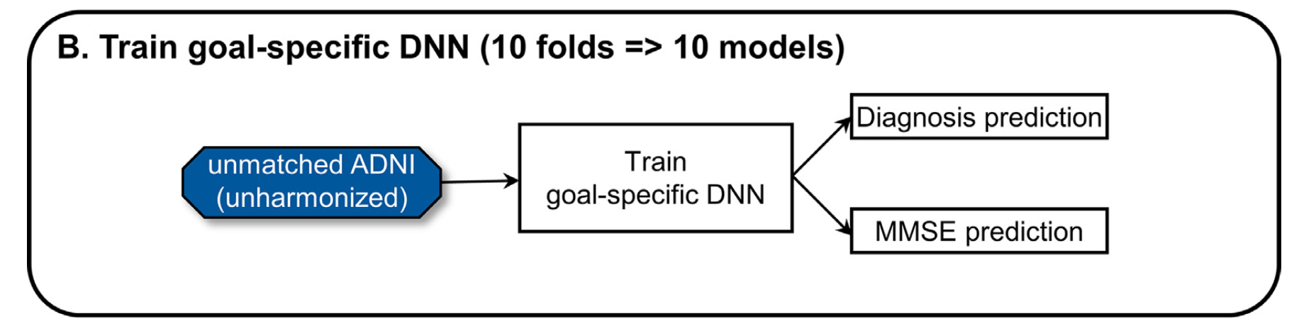Figure 5: Training of goal-specific DNN. The downstream application includes diagnosis and MMSE prediction [5]

The DNN outputs a diagnosis prediction (a classification task) and an MMSE prediction (a regression task). Diagnosis prediction includes 3 classes: normal controls, mild cognitive impairment (MCI), and Alzheimer’s disease dementia (AD). MMSE is the Mini-Mental State Examination score.

After the goal-specific DNN is trained, we input the reconstructed x from a trained cVAE to the goal-specific DNN, and finetune the trained cVAE with goal-specific DNN frozen, as shown in Figure 6:

Figure 6: Architecture of gcVAE

The loss function is the weighted sum of the loss for two prediction tasks:

where MAE is the mean absolute error of MMSE prediction, and CrossEntropy is the cross entropy loss for diagnosis prediction. α_MMSE and α_DX are their corresponding weights.

3.4 Training Setting

First datasets should be matched with age, sex, MMSE, and diagnosis to get matched pairs. The authors use matched data for evaluation, and unmatched data to train. There are mainly two reasons:

1. matched data is much less than unmatched data
2. ensure the prediction performance is comparable, i.e. any difference in prediction is caused by unavoidable dataset differences

Let's explain the second reason more closely. Suppose the diagnosis for ADNI and AIBL datasets are composed as follows:

• ADNI: 45% normal, 45% AD, 10% MCI
• AIBL: 33% normal, 33% AD, 33% MCI

Because normal cases and AD cases are easier to predict than MCI, the prediction performance of ADNI would likely be better than AIBL, which may act as a confounder in prediction tasks. 

The matching process is shown in Figure 7:

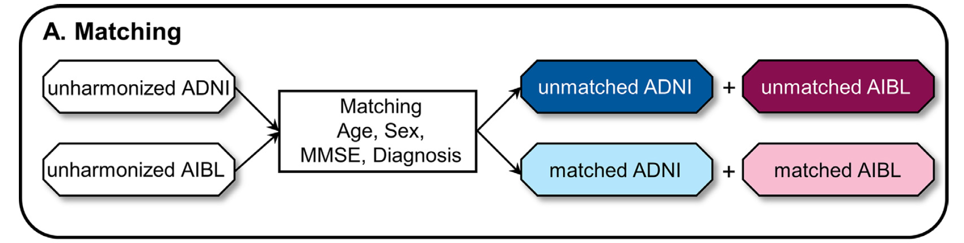Figure 7: Matching process [5]

We then train a goal-specific DNN as shown in Figure 5. Further, we train two baseline harmonization models ComBat and cVAE, together with the proposed gcVAE, as shown in Figure 8:

Figure 8: Training of harmonization models [5]

After training harmonization models, we apply them to all datasets and get harmonized datasets.

3.5 Evaluation Setting

The evaluation setting is shown in Figure 9:

Figure 9: Evaluation of harmonization models [5]

• Dataset prediction: First train an XGBoost classifier using unmatched harmonized ADNI and unmatched harmonized AIBL data, and test the classifier using matched harmonized ADNI and matched harmonized AIBL data. Lower dataset prediction acc indicates more dataset differences removal.
• Downstream application performance: Apply trained goal-specific DNN to three datasets with matched participants. Here we are interested in how good it is to map AIBL to ADNI, so the two unharmonized datasets serve as control groups, and harmonized AIBL is the experimental group.

The reason why we need downstream application performance except for dataset prediction evaluation is to avoid trivial solutions in dataset differences removal, i.e. loss of biological information. For example, the harmonization models simply map all data to zero vectors.

4. Experimental Results

Core results include dataset prediction accuracy and downstream application (diagnosis prediction + MMSE prediction), as shown in Figure 10:

Figure 10: Results from the paper [5]. Columns from left to right represent results of dataset prediction accuracy, diagnosis prediction, and MMSE prediction

1. The table on the right side of the results shows whether there is a statistical difference, while * indicates there is a significant statistical difference (great improvement or reduction) and n.s. means not significant
2. Dataset prediction accuracy (1st column): Accuracies of cVAE and gcVAE are significantly lower than ComBat in ADNI-AIBL experiment, which means they remove more dataset differences than ComBat. however, they are still better than chance, suggesting residual dataset differences. Similar results are shown in ADNI-MACC experiment.
3. Diagnosis prediction accuracy (2nd column): gcVAE yields the best acc, even better than unharmonized ADNI, which should be the upper bound for harmonized datasets because no information is lost. The reason provided by the author is that the weights for the goal-specific DNN might have favored diagnosis prediction more than MMSE in the case of AIBL. While in ADNI-MACC, gcVAE is better than ComBat and cVAE while still worse than unharmonized ADNI. Another reason could be that the harmonized images provided by gcVAE change a lot from their original appearance, which means the diagnosis prediction improves at the expense of no longer being suitable to provide to physicians for diagnosis.
4. MMSE prediction MAE loss (3rd column): In ADNI-AIBL, gcVAE is better than cVAE, and there is no statistical difference among Combat, unharmonized AIBL, and gcVAE. But gcVAE is still worse than unharmonized ADNI, which indicates room for improvement. In ADNI-MACC, similar results are shown but gcVAE yields competitive MAE to unharmonized ADNI.

5. Discussion

The proposed gcVAE makes use of downstream applications to guide the harmonization process, which enables it to preserve biological information while removing site differences, as shown in results from three large-scale MRI datasets. Another advantage is that this goal-specific framework can easily be applied to any NN-based methods because we just need to fine-tune our harmonization model on downstream tasks.

However, there are also drawbacks to this method. As mentioned by the authors, the biggest shortcoming is that it's not generalizable to new downstream applications, which means that when we encounter another downstream application, we have to retrain our harmonization model. It would be very inefficient and computationally expensive. From my perspective, this method can be sensitive to pretrained networks. Because two networks have to be trained beforehand, i.e. the goal-specific network and cVAE, and if we don't train them well, which means the optimization is not good enough, our trained gcVAE is unlikely to perform well. One more obvious drawback is that this method cannot apply to non-NN-based methods.

Personally, I like how the training and evaluation are designed because they're logically rigorous by considering so many factors like confounders and shortcut solutions in evaluation. But I'm still not convinced by the explanations of the results of diagnosis prediction (2nd column in Figure 10). The authors argue that gcVAE outperforms unharmonized ADNI due to preference of weights in goal-specific DNN, in this case, why not train two separte networks for diagnosis prediction and MMSE prediction? After all, despite of the close correlation between MMSE score and AD diagnosis, these two tasks are quite different in that one is regression task and the other is classification task. Unfortunately no explanation is given in the paper concerning why we should combine these two tasks in a single network.

6. References

[1]: Zuo, Lianrui, et al. "Unsupervised MR harmonization by learning disentangled representations using information bottleneck theory." NeuroImage 243 (2021): 118569.

[2]: Johnson, W. Evan, Cheng Li, and Ariel Rabinovic. "Adjusting batch effects in microarray expression data using empirical Bayes methods." Biostatistics 8.1 (2007): 118-127.

[3]: Zhao, Fenqiang, et al. "Harmonization of infant cortical thickness using surface-to-surface cycle-consistent adversarial networks." Medical Image Computing and Computer Assisted Intervention–MICCAI 2019: 22nd International Conference, Shenzhen, China, October 13–17, 2019, Proceedings, Part IV. Cham: Springer International Publishing, 2019.

[4]: Moyer, Daniel, et al. "Scanner invariant representations for diffusion MRI harmonization." Magnetic resonance in medicine 84.4 (2020): 2174-2189.

[5]: An, Lijun, et al. "Goal-specific brain MRI harmonization." NeuroImage 263 (2022): 119570.

[6]: https://surfer.nmr.mgh.harvard.edu/