Authors : Li Xiao , Junqi Wang, Peyman H. Kassani, Yipu Zhang , Yuntong Bai , Julia M. Stephen , Tony W. Wilson , Vince D. Calhoun, Fellow, IEEE, and Yu-Ping Wang , Senior Member, IEEE
Blog author : Alina Weinberger
The brain is a network
In understanding the brain, it is crucial to investigate the relationship between structure and function. Neuroscience research has established a very detailed map of distinct anatomical regions that have different functional roles, but to understand how behaviour is generated, it seems neuronal activity needs to be considered in terms of networks, for example by studying the connectivity between different anatomical regions (Pessoa, 2014).
For that, one needs multiple tools: data, an analytical framework, and a measure of connectivity.
The data : FMRI
Magnetic resonance imaging (MRI), takes advantage of magnetic inhomogeneities generated by our body, measured inside a device that generates a huge magnetic field. This enables us to build a detailed anatomical atlas of our brain. Its cousin, functional magnetic resonance imaging (fMRI), specifically determines the magnetic inhomogeneities generated by the oxygen-carrying blood particles hemoglobin. Assuming very active brain regions will consume a lot of oxygen, we will observe a relative increase of deoxyhemoglobin (the hemoglobin depleted of oxygen) at that site, which will generate an increased signal. This signal called the blood oxygen level-dependent (BOLD) contrast, is recorded over time and is considered a good proxy of brain activity over time (Whitten, 2012). Yet, even if we can guess which regions are active, we don't know how they are connected to form a network!
The framework : Graph theory
Simple graphs
Analyzing connections between nodes is a whole mathematical field of research: graph theory. Nodes, also called vertices, are connected by edges, that might have a weight (indicating the strength of the connection). One example is given below:

| (1) | G = \{V, \Epsilon\} \text{ where } V = \{V1, V2, V3\} \text{ and } E = \{E1, E2, E3\} |
Together, those elements form a simple graph, that can be equivalently characterized in multiple ways. Particularly, matrices where the rows and columns represent vertices and edges, respectively, (called an incidence matrix H), can be used to uniquely define the graph. The incidence matrix below, for example, is equivalent to the graph above:

\[
H_{ij}=\left\{
\begin{array}{ll}
1 \textit{, if $v_{ij} \in \Epsilon$ }\\
0 \textit{, otherwise} \\
\end{array}
\right.
\]
Hypergraphs
One extension of that is the so-called hyper-graph. One edge, instead of connecting only two edges, can connect an arbitrary number of nodes, and is therefore called a 'hyper-edge'. It is then represented as a circle or ellipse around the nodes connected by that edge. Similar matrices can be used to represent that graph, as shown below:

Vertex degree and edge degree
The vertex degree (number of edges connected to a vertex), and the edge degree (number of vertices connected to that edge) can then be defined from the incidence matrix H by simply summing over the rows or columns:
| (2) | d(v_i) = \sum_{e_j \in E} w(e_j) \cdot H_{ij} |
| (3) | d(e_i) = \sum_{v_i \in V} H_{ij} |
We can then define D_v = diag(d(v_1), d(v_2),..., d(v_N) and D_e = diag(d(e_1), d(e_2),..., d(e_N) the diagonal matrices of vertex and hyper edge degrees.
Laplacian
The graph laplacian can be defined by the difference between the edge degree matrix and some matrix representing connectivity in the graph. Most commonly, one uses the adjacency matrix to do so (where columns and rows are the vertices, and entries are only non-zero if those vertices are connected), but the authors of the paper chose a different method. Here, the laplacian is defined with a so-called similarity matrix, where entries take into account the incidence, the weights of the connection and the edge degree.
| (4) | L_S = D_{e} - S |
were
| (5) | S = HWD_{e}_{-1}H_{T} |
is a matrix that represents a pair-wise similarity measure between the nodes.
The Laplacian will be a central element in learning the edges and weights of our graph, as we will see a bit further.
Commonly used methods to compute functional connectivity
Functional connectivity refers to the statistical dependence or correlation between different brain regions, so-called regions of interest (ROIS). Note that functional connectivity does by definition not take into account the direction of the connection (ref assessing fmri), so graphs that can be obtained with this measure are non-directional. Different methods can be employed to determine these relationships, which are then represented as a graph. Let's discuss some traditional approaches first.
Pearsons correlation
One straightforward approach is to calculate the pairwise correlation between the activity of the ROIs. This approach is very computationally expensive since the number of regions of interest in the 3D volume of the brain can be as much as hundreds of thousands. A simple solution to that problem can be to predefine one region, the so-called 'seed', that is assumed to be relevant and compute all correlations between that node and every other node in the brain. The disadvantage of that method is that it relies on an expert opinion on which region might be relevant in the first place. Regions that have a statistically significant dependence are then considered 'connected' (Rogers et al., 2007), and this connection is represented by the existence of an edge between these regions in our built graph.
Dimensionality reduction - Principal components analysis
This method includes a dimensionality reduction step before computing the correlation between regions. The eigenvalue decompositions allow to extract vectors corresponding to the direction of the maximum variance of the data.PCA ranks the components based on their contribution to the total variance in the data, with the first component capturing the most variance, the second capturing the next largest, and so on. After selecting a certain number of components, the components are projected back to the original space and the same statistical analysis as described above is performed. Using PCA for functional connectivity analysis can help reveal the major modes of brain activity and identify intrinsic connectivity networks without relying on a priori-defined regions of interest, but the interpretation of the found components can be challenging or even impossible (Rogers et al., 2007).
Graph learning
Graph signal processing is an emerging field that has initially developed for the study of a wide range of networks, going from traffic networks to communications. Also in our case, this enables a data-driven approach to investigate brain connectivity. One important assumption made here is that the signals in each node change smoothly between connected nodes in the network. We will explain this concept in more detail a bit later.
Learning the edges - Sparse linear regression (the Lasso)
Sparse linear regression is a technique that combines linear regression with sparsity-inducing regularization to learn the edges or connections in a graph from observed data. By promoting sparsity, it automatically selects the most significant edges, facilitating the discovery of the underlying graph structure. (ChatGPT) More formally:
| (6) | min_{\alpha_i} \frac{1}{2} ||x_i - A_i \alpha_i ||_2^2 + \lambda ||\alpha_i||_1 |
Here, we assume that nodes are connected if the signals in one node can be represented as a linear combination of the connected node, by finding the coefficients\alpha_i which best explain the data. Only connections with non-zero and positive coefficients are kept, and these connections become part of our edge set. Next, we want to compute the corresponding weights.
Learning the weights - smoothness of the signal
Borrowing the concept of smoothness from signal processing, the concept of a smooth signal on a graph can be defined.
Let f = (f_1, f_2,... f_N)^T be an arbitrary signal on the vertices of a graph G (this would represent our time-varying fMRI signal on each ROI we have previously defined), then the smoothness on the signal is defined as
| f_tLf = \frac{1}{2} \sum_{i=1}^{N}\sum_{j=1}^{N} S_{ij} (f_i - f_j)^2 |
which is also called the Laplacian quadratic form. This measure indicates how well a signal 'fits' on a graph, specifically, how smoothly the signal changes in well-connected nodes on the graph. In other words, if the values in well-connected nodes are similar over time, the signal is smooth on graph G. This is illustrated in the graph below. Consider the red bars to be positive signal values, the blue bars as negative signal values, and the length of the bar as the signal intensity. Conceptually, the signal being smooth on the graph means that the nodes with positive signals should be strongly connected, and nodes with negative signals should be strongly connected, but not so much between them.

This can be then used as an objective function to optimize the weights of the graph we are trying to learn by maximizing this smoothness function in the following way:
\begin{array}{ll}
\min _{\mathbf{w}} & \operatorname{tr}\left(\mathbf{X}^T \mathbf{L} \mathbf{X}\right)+\rho\|\mathbf{w}\|_2^2 \\
\text { s.t. } & \mathbf{w} \succeq 0 \\
& \|\mathbf{w}\|_1=1,
\end{array}
From the weights that are learned this way, we can construct the similarity matrix as defined before. This similarity matrix can then be used as a feature for classification, for example, as in this paper, using a simple SVM classifier.
To summarize, the procedure looks as follows: 
The procedure above enables the extraction of a biologically meaningful brain network from fMRI data, that can further be used to distinguish different populations. In the case of our paper, the high WRAT score and low WRAT score groups were classified.
Going even further - Multi hyper-graphs
What if we could make use of multiple fMRI paradigms at the same time, to extract even more meaningful information from our data? This is exactly what the authors tried to do here: constructing a unified multi-hypergraph containing information about different fMRI paradigms. Let's take a closer look at their methods.
The unified incidence matrix H
First, they computed one incidence matrix per paradigm and concatenated those. This is what they call an 'unified' incidence matrix H, formally defined as H = (H^{(1}, H^{(2}, ..., H^{(N} ).
The unified weight vector w
Next, they are trying to learn the optimal weights for each paradigm, using the incidence matrices of all paradigms. Remember that the Laplacian matrix is computed using the similarity matrix, which in turn contains the incidence matrix. The matrix X contains all the signals of one particular fMRI paradigm. Therefore, the smoothness of the signal of one particular fMRI paradigm is optimized on a graph built using all paradigms.
\begin{aligned}
& \min _{\mathbf{w}} \frac{1}{K} \sum_{k=1}^K \operatorname{tr}\left(\left(\mathbf{X}^{(k)}\right)^T \mathbf{L}^{(k)} \mathbf{X}^{(k)}\right)+\rho\|\mathbf{w}\|_2^2 \\
& \text { s.t. } \quad \mathbf{w} \succeq 0 \\
& \quad\|\mathbf{w}\|_1=1
\end{aligned}
The obtained weight vectors are then concatenated one more time, to forme the unified weight vector w, as follows : w = (w^{(1}, w^{(2}, ..., w^{(N} ).
The unified similarity matrix S
Finally, the similarity matrix is computed
$$
\mathbf{S}=\mathbf{H W D}_e^{-1} \mathbf{H}^T=\sum_{k=1}^K \mathbf{S}^{(k)}
$$
where\left.\left.\mathbf{W}=\operatorname{diag}(\mathbf{w}), \mathbf{D}_e=\operatorname{diag}\left(\mathbf{D}_e^{(1)}\right), \mathbf{D}_e^{(2}\right), \cdots, \mathbf{D}_e^{(K)}\right), and\mathbf{S}^{(k)}=\mathbf{H}^{(k)} \mathbf{W}^{(k)}\left(\mathbf{D}_e^{(k)}\right)^{-1}\left(\mathbf{H}^{(k)}\right)^T denotes the hypergraph similarity matrix for the k-th fMRI paradigm and used as input for an SVM classifier.
Visually, the procedure can be represented as follows:

Data
The freely available dataset from the PCN project (Satterthwaite et al., 2014), where 900 adolescents underwent different fMRI paradigms and cognitive testing was used to test the feature extraction method above. These tests included the WRAT score, which measures learning abilities such as reading recognition, spelling, and math computation. Data from adolescents that underwent a resting state task, an emotion recognition task and a stimulus-response task (n-back test), were kept for further analysis. After computing the hyper networks and multi-hyper networks on those, classification based on a high vs low WRAT score of the participants was performed. The dataset can be downloaded freely from the DbGaP study website.
Results
As mentioned before, the hyper-networks and multi-hyper networks extracted from each participant hopefully represent the actual brain network responsible for the cognitive abilities tests during the fMRI tasks. Therefore, 2 outcomes are desired here:
- First, the classification using the aforementioned networks should be more accurate than using other feature extraction methods
- Second, the extracted network should be biologically plausible, i.e. contain brain regions that have previously been associated with cognitive reasoning and learning ability
Classification accuracy
To assess how well the classifier could distinguish between the high or low WRAT score group based on the hyper networks extracted from the FMRI data, they compared this method to the following competing methods:
- PC : Pearson’s correlation method
- GLasso : partial correlation method with the graphical Lasso
- UW-Lasso : unweighted hypergraph-based method with the incidence matrix being calculated by the Lasso
- UW-WLasso : unweighted hypergraph-based method with the incidence matrix H being calculated by the weighted Lasso
- UW-ElasticNet : unweighted hypergraph-based method with the incidence matrix H being calculated by the Elastic Net
Let's have a look at the results:
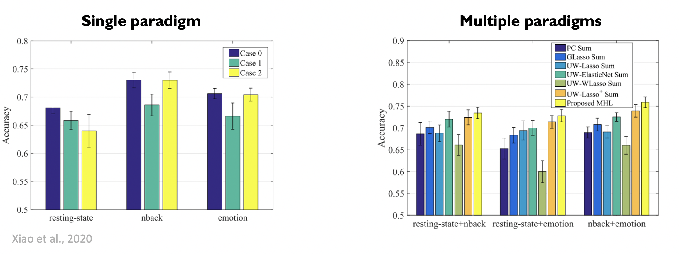
It is clear that the proposed multi-hyper network outperforms the other methods, and also outperforms the signal paradigm method, where they only compute the graph on the data of a single fMRI task per subject.
Interpretability
Most discriminative brain regions
Here is a plot with the brain regions that were the most discriminative ROIs in most subjects. In other words, these were the brain regions mostly recognized as having a different activity in subjects performing well at cognitive tasks, versus this who performed less well.
 Notably, a lot of frontal regions seem to be particularly discriminative..The superior frontal gyrus is very important for working memory, decision making and impulse control (Hu et al., 2016). However, it seems like most of the highlighted regions are at least partially language-related. For example, the inferior frontal gyrus is involved in inhibition and attentional control (Hampshire et al., 2010), but also contains Broca's area, very well known to be involved in language production (Chang et al., 2015). Also, temporal areas are known to be involved in auditory processing (Moore, 1991). The posterior cingulate gyrus is highly involved in emotional processing and therefore liked to reward generating behaviour, but also seems to be linked to internal cognition during a resting state condition (Leech & Sharp, 2013).
Unfortunately, the authors did not mention from which of the conditions this graph was computed.
- Most discriminative connections
The authors performed a two sided-test to find out which of the connection were most discriminative. Let's have a deeper look here as well.

We can see that connection from the frontal cortex to temporal regions seems to be very important here. For example, the connection between the superior frontal gyrus and the insult is known to be part of a broader network that plays a key role in decision-making, but also in emotional regulation and self-awareness. The superior frontal gyrus and the angular gyrus are both part of a working memory and language processing network. The middle frontal gyrus and the precuneus are part of the default mode network, known to be involved in self reflection and daydreaming (chatGPT).
The presence of the Crus 2 node in the cerebellum is very interesting. The cerebellum has been thought to be involved in fine-tuning motor commands only for a long time, but recently, finding about the involvement of the cerebellum in cognition have emerged. Particularly, the connection between this nucleus and the middle temporal gyrus is part of a higher-order cognitive network, that participates in semantic cognition and language processing (chatGPT).
Discussion
Benefits
Hypergraphs - Higher order relations
Constructing accurate brain networks is crucial in understanding the complex organization of the brain. Existing methods often use simple graphs, limiting their ability to capture higher-order relationships among multiple regions of interest (ROIs). The approach of the authors involves generating hyper-edges using sparse linear regression, connecting any number of ROIs, and determining hyperedge weights through hypergraph learning, allowing to capture of high-order relationships and resulting in more informative and discriminative features compared to existing methods.
Multi-hypergraphs - combining information from multiple paradigms
By integrating information from multiple fMRI paradigms, this method also improves classification performance compared to traditional graph-based methods and existing unweighted hypergraph approaches.
Complexity
Unlike traditional deep learning methods that require a large number of parameters and extensive training, the proposed method achieves this without introducing excessive parameters. This approach allows for more easy interpretation, mitigates overfitting issues, and enhances generalization capabilities, particularly in scenarios with limited sample sizes, as it is way too often the case in neuroscience research.
Limitations
Decoding accuracy
The highest decoding accuracy was about 75%, which is not enough for an independent medical diagnosis system. However, it can be used as a complementary tool for a clinician or to point an investigator in the right direction to investigate a particular network better.
Anatomical information
Structural connectivity information was not incorporated for the construction of the networks. Functional connectivity solely based on statistical relationships between brain regions does not account for the underlying anatomical connections. Structural connectivity, which represents the physical connections between brain regions, plays a crucial role in shaping functional interactions. Ignoring structural information can lead to misinterpretation and an incomplete understanding of functional connections.
On the combination method of multiple paradigms - my personal comment
The paradigms that the authors choose to combine were a resting state, an emotion recognition task and an n-back test. In my opinion, these are very different networks and the default mode network, active in resting state tasks, is actually known to be suppressed by any active task, such as emotion recognition and stimulus-response tasks. Therefore, if we consider the paradigms pairwise (resting-state, emotion recognition) and (resting state, n-back), those networks are not complementary but opposite.
When we analyze more closely the way the authors constructed the 'unified' weight matrices and similarity matrices, the mathematical tools they seem to have chosen are concatenation and summation.
Recall how the 'unified' hyper edge weight vector is computed: First, the incidence matrices for each paradigm are computed separately, then they are concatenated. By construction, the matrices of the resting state paradigm and the emotion or stimulus-response task will be sparse, and the entries of the resting state incidence matrix will be non-zero at completely different indices than the other two tasks. The next step is to calculate the hyperedge weight, and as one can read out of the formula, the weight vector of each paradigm is calculated by minimizing the sum of the loss function over all paradigms. This will inevitably lead to confusion between relevant edges for the resting state task (the default mode network), and the other two tasks (active cognitive processing). It can be argued that indeed, the classification accuracy got better by combining the different paradigms, as shown in the result section of the paper. However, this interpretability part of this computed hyper-network suffers from the chosen methodology. As noted in the most discriminative regions and connection section, some of those regions are involved in cognitive processing, some in emotional processing, and some with sensory processing. As these are biologically different networks, constructing a graph that tries to fit all of them at the same time cannot result in a biologically plausible network.
Conclusion
In their paper, the authors introduced a (multi-)hypergraph learning-based method inspired by recent research. Their approach involved constructing a weighted hypergraph where hyperedges were generated using sparse representation, and hyperedge weights were learned through (multi-)hypergraph learning. They then defined a hypergraph similarity matrix to represent the functional connectivity network (FCN). Unlike traditional graph-based methods that only capture pairwise relationships between regions of interest (ROIs), their proposed method characterizes high-order relationships among multiple ROIs using the hypergraph similarity matrix, providing valuable insights into complex brain networks. The effectiveness of their method in predicting WRAT scores was evaluated using fMRI data from the PNC, involving three paradigms. Experimental results demonstrated the superiority of their approach over traditional graph-based methods and existing unweighted hypergraph-based methods. Additionally, their method provided additional information about the underlying biomarkers of the networks associated with the WRAT score, but the interpretation is to be taken with caution here. An important next step would be systematically comparing the connections found by this method and the existing literature. Also, another method of combining the different paradigms should be considered, focusing on biological interpretability.
References
Literature
Chang, E. F., Raygor, K. P., & Berger, M. S. (2015). Contemporary model of Language Organization: An overview for neurosurgeons. Journal of Neurosurgery, 122(2), 250–261. https://doi.org/10.3171/2014.10.jns132647
Hampshire, A., Chamberlain, S. R., Monti, M. M., Duncan, J., & Owen, A. M. (2010). The role of the right inferior frontal gyrus: Inhibition and attentional control. NeuroImage, 50(3), 1313–1319. https://doi.org/10.1016/j.neuroimage.2009.12.109
Hu, S., Ide, J. S., Zhang, S., & Li, C. R. (2016). The right superior frontal gyrus and individual variation in proactive control of impulsive response. The Journal of Neuroscience, 36(50), 12688–12696. https://doi.org/10.1523/jneurosci.1175-16.2016
Leech, R., & Sharp, D. J. (2013). The role of the posterior cingulate cortex in cognition and disease. Brain, 137(1), 12–32. https://doi.org/10.1093/brain/awt162
Moore, D. R. (1991). Anatomy and physiology of binaural hearing. International Journal of Audiology, 30(3), 125–134. https://doi.org/10.3109/00206099109072878
U.S. National Library of Medicine. (n.d.). DbGaP study. National Center for Biotechnology Information. https://www.ncbi.nlm.nih.gov/projects/gap/cgi-bin/study.cgi?study_id=phs001672.v8.p1
Pessoa, L. (2014). Understanding brain networks and brain organization. Physics of Life Reviews, 11(3), 400–435. https://doi.org/10.1016/j.plrev.2014.03.005
Rogers, B. P., Morgan, V. L., Newton, A. T., & Gore, J. C. (2007). Assessing functional connectivity in the human brain by fmri. Magnetic Resonance Imaging, 25(10), 1347–1357. https://doi.org/10.1016/j.mri.2007.03.007
Satterthwaite, T. D., Elliott, M. A., Ruparel, K., Loughead, J., Prabhakaran, K., Calkins, M. E., Hopson, R., Jackson, C., Keefe, J., Riley, M., Mentch, F. D., Sleiman, P., Verma, R., Davatzikos, C., Hakonarson, H., Gur, R. C., & Gur, R. E. (2014). Neuroimaging of the philadelphia neurodevelopmental cohort. NeuroImage, 86, 544–553. https://doi.org/10.1016/j.neuroimage.2013.07.064
Whitten, L. (2012). Functional Magnetic Resonance Imaging (Fmri): An Invaluable Tool in Translational Neuroscience. https://doi.org/10.3768/rtipress.2012.op.0010.1212
Images
Simple graph and incidence matrix: Terms related to graphs. Networks. (n.d.). https://networkgraph.weebly.com/terms-related-to-graphs.html
Smoothness on a graph: YouTube. (2018, July 27). Xiaowen Dong: Learning graphs from data: A Signal Processing Perspective. YouTube. https://www.youtube.com/watch?v=2ds4A11DSOw
ChatGPT prompts
- Explain sparse linear regression to learn weights in the context of graph learning
- What is the function of (brain region X)
- Are the (brain region X) and the (brain region Y) connected in the brain and if yes, what is the function of this connection
- Is the nucleus crus 2 of the cerebellum involved in cognitive processes
- Reformulate the following text in 3 sentences: (text)