Introduction
Rajat Talak et al. start off by elaborating on the limited expressiveness of standard graph neural network (GNN) architectures. Models such as CPNGNN [1] and DimeNet [2] lack the power to capture basic graph properties such as the girth, the circumference, and the diameter of a graph [3]. Efforts to improve upon these architectures are mostly theoretic and intractable in practice. It is suggested that graph neural networks should at least possess the power to model any probabilistic graphical model (PGM). Exact inference of such models, a problem proven to be NP-hard, is beyond the capabilities of standard GNN architectures as well. Contributions by the authors are twofold:
- The introduction of G-compatibility, arguing that the approximation of a G-compatible function is equivalent to the approximation of any probability distribution on a PGM.
- The proposition of the Neural Tree (NT) architecture, which they prove capable of such an approximation.
Experiments on instances of two classes of graphs, 3D scene graphs and citation networks, show the substantial improvement delivered by NTs over contemporary architectures.
Methodology
Preliminaries & Definitions
Node classification and semi-supervised learning. Let G=(V,E) be a graph with the set of vertices V and a set of edges E. Let all vertices of this graph have a vector of features \mathbf{X} = (\mathbf{x}_v) associated with it. In node classification, the task is to assign labels y_v, elements of a finite set of classes, to a node v. As is the focus of this paper, semi-supervised learning is concerned with the inference of labels with the twist that the training data does not provide an exhaustive ground truth: Only a subset A \subset V is labeled.
Graph Neural Network. In standard graph neural network architectures, node features are iteratively aggregated in a neighborhood according to the following computation prescription:
| h^t_v=AGG_t(h^{t-1}_v,\{(h^{t-1}_u,\kappa_{u,v})\ |\ u \in N_G(v)\}) |
The initial value of the embedding of any given vertexh^0_v is \mathbf{x}_v. The function N_G(v) describes the neighborhood of v, and \kappa_{u,v} is a learnable parameter associated with the edge (u, v). Aggregating information from the neighborhood of a vertex is referred to as message passing and will become relevant again later. The recursive computation of embeddings h^t_v is repeated for a number of iterations T and the final prediction is modeled as
| y_v = READ(h^T_v) |
. Both AGG_t and READ are modeled as single or multi-layer perceptrons.
G-Invariant function. A function f : \mathbb{R}^m\to\mathbb{R}^n is called graph invariant if it satisfies f (\varphi (g) \cdot x) = f ( x )\ \text{for all}\ x \in \mathbb{R}^n\ \text{and}\ g \in G and a homomorphism \varphi : G \to S_m [8].
G-Equivariant function. A function f: \mathbb{R}^m \to \mathbb{R}^n is called graph equivariant if it satisfies f (\varphi (g) \cdot x) = \psi(g) \cdot f ( x )\ \text{for all}\ g \in G and a homomorphism \psi : G \to S_n.
G-Compatible function. A function f:(\times_{v \in V}\mathbb{X}_v,G)\to\mathbb{R} is compatible with a graph G if it can be factorized as
| f(\mathbf{X})=\sum_{c \in C(G)}\theta_c(\mathbf{x}_C)} |
. Here, C(G) denotes the set of all maximal cliques – a complete subgraph of G is called a clique – in G and \theta_c maps \times_{v\in c}\mathbb{X}_v – the set of node features in the clique c – to a real number.
Rajat Talak et al. further show that any continuous scalar graph invariant function can be \epsilon -approximated via non-linear combinations of graph compatible functions and that the same result holds for any vector-valued graph equivariant function (i.e. it's components) w.l.o.g. This means that the NT architecture will not only be useful in the approximation of the probability distributions in PGMs, but also when it comes to the approximation of graph invariant / equivariant functions.
Treewidth. The treewidth of a tree decomposition of a graph is the size of the largest bag (i.e. a subset of the graph's nodes) of the tree minus one.
The Neural Tree Architecture
The neural tree architecture is a modular design that can be combined with message passing neural networks. The core data structure is the so-called H-tree which is a tree-like representation of a graph and its sub-graphs. One can construct an H-tree by recursively performing tree composition on a graph and merging the results of recursive calls:
Given is the following input graph:

Step 1: Perform tree decomposition on the input graph. The following figure shows the junction-tree decomposition [5] (the algorithm chosen by the authors) of the input graph:

Step 2: Identify the subgraphs induced by the bags of the junction-tree:

Step 3: Apply tree decomposition recursively to the subgraphs: The first recursive call yields:

Step 4: Hierarchically combine results and remove the edges connecting the root nodes of the subgraphs' H-trees to avoid cycles. Merging the results of the recursive calls yields the following trees:

Merging these sub-trees back into the junction-tree of the input graph yields the final H-tree (removed edges between root nodes of sub-trees are drawn dashed red):

As the figure above suggests, all vertices of the input graph have a corresponding leaf node in the resulting H-tree. Let \kappa(l) be the node in the input graph that corresponds to the leaf node l in the H-tree. The leaf l will receive the feature \mathbf{x}_v if \kappa(l)=v. All other features are set to \mathbf{0}. Subsequently, one can use any message passing GNN architecture to learn on the H-tree, as it is a regular graph. Novel in the NT architecture is that inference is performed only on the leaf nodes of the tree, as those represent the nodes in the input graph that are to be classified. Mathematically speaking, this means
| y_v=COMB(\{h^T_l\ |\ l\ \text{leaf node in}\ J_G\ \text{s.t.}\ \kappa(l)=v\}) |
instead of
| y_v = READ(h^T_v) |
. Which and how many parameters need to be learned depends on the implementation of the message passing and aggregation function.
Substantial Remarks
- Performing tree decomposition on a graph has exponential time and space complexity in the treewidth of G. By sub-sampling G before constructing the H-tree, the NT architecture remains tractable for problems with high treewidhts such as citation networks.
- The number of parameters is linear in the number of nodes in G and exponential in its treewidth.
- If the training set contains graphs with an average treewidth that is small enough, the amount of traning data required also scales linearly with the number of nodes.
Experiments
Approaches and Datasets
The authors applied the NT architecture to node classification in 3D scene graphs and citation networks.
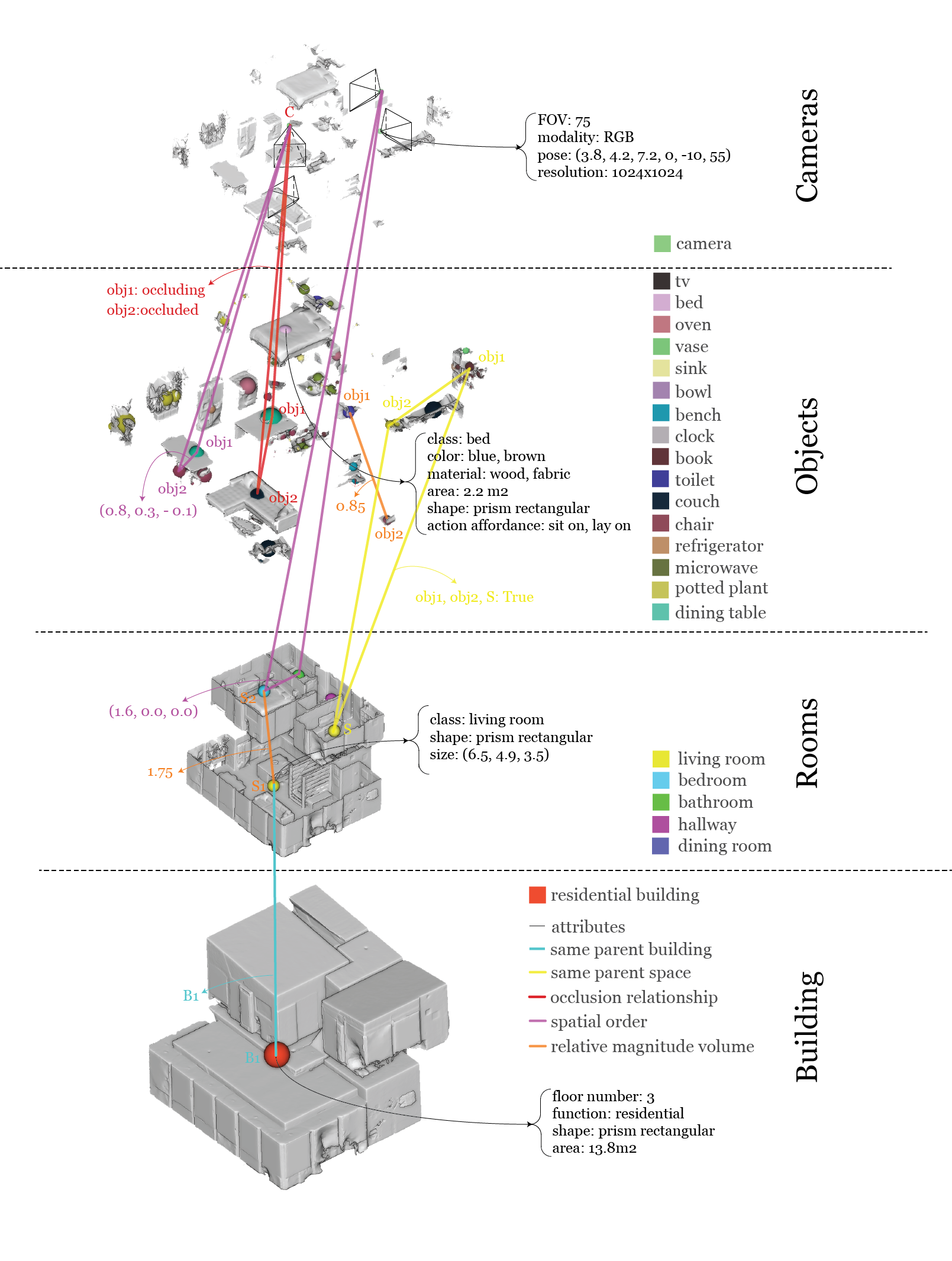
3D scene graph dataset. For the former they used the 3D scene graph dataset by Stanford which contains 35 scene graphs including labels for buildings, rooms, and objects. As there is only one label for the building class, these nodes are discarded, thus yielding 482 graphs representing only the rooms (15 possible labels) and the objects (35 possible labels) contained therein. The authors further added 4920 edges between object nodes, though they do not elaborate on their intention behind this. The goal might have been to add relations between objects in rooms since that proved to increase inference accuarcy. The node features are chosen as the geometrical center and the bounding box dimensions of an object or a room. For the implementation of the aforementioned AGG_t function, an implementation as specified in GCN, GraphSAGE, GAT, and GIN is used. As for the test split, 70% of the nodes were used for training, 20% for validation, and 10% for testing.
Citation network datasets. The authors used CiteSeer, Cora, and Pubmed, similar to Yang et al. in "Revising semi-supervised learning with graph embeddings" [6]. In these sets, the nodes are documents and citations are represented by undirected edges. Any document's subject is the target label of the corresponding node. The fact that NTs have exponential complexity in the treewidth poses a disadvantage in the case of citation networks, which commonly have a high treewidth. Rajat Talak et al. show that the application of this architecture is tractable for this problem class by first performing bounded treewidth graph sub-sampling [7] on the input graph before constructing the H-tree. To provide some insights into the magnitude of the mentioned datasets: The CiteSeer citation network contains over 380.000 nodes and more than 1.751.000 edges. The nodes have an average degree of ~9, with some nodes having a degree of over 1900! [9].
Results
3D scene graph. Figures for the experiment on 3D scene graphs in Table (1) – an averaged performance over 100 runs – indicate a clear improvement over "competing" architectures. The NT architecture outperforms GCN, GAT, and GIN by more than 12% on average, while the improvement upon GraphSAGE was found to be roughly 4%. An interesting takeaway from the direct comparisons between GCN and GCN performed on a NT are illustrated in Figure (4): Test accuracy increases up to an optimum and rapidly declines afterwards.
As with the number of iterations T , we see an optimal T at which the test accuracy is maximized. This optimal T is empirically close to the average diameter of the constructed H-trees, of all (room-object) scene graphs in the dataset. This is intuitive, as for the messages to propagate across the entire H-tree, T would have to equal the diameter of the H-tree.
It is worth noting that, according to the author's findings, the neural tree approach only becomes superior to standard models after a certain size of training data. After this threshold is hit, however, a model combining a NT and GCN – the case illustrated in the paper – consistently outperforms standard GCN.


Citation networks. Discussion on the performance in the main article was limited. The authors only mentioned the tests of the NT with a GCN on the Pubmed dataset, though the supplementary material contains further details. Recall that the input graph was sub-sampled before being decomposed in order to reduce its treewidth. This bound is a hyperparameter, and Figure (5) shows that this parameter can be chosen as small as k=1 with little to no impact on the accuracy. Again, performing message passing on the H-tree has lead to more accurate inference if given sufficient training data.

Figure (5) also shows how the neural tree architecture scales with data: Whereas the improvement of NT+GCN over GCN was ~10% in the experiment on the 3D graph dataset, the improvement of graph-subsampling+NT+GCN over GCN was a mere ~3% for the Pubmed citation network. While the NT still outperforms standard architectures on graphs with nodes and edges in the hundredths of thousands, the increase in accuracy is way more noticable in the experiment using a graph with significantly fewer nodes and edges (in the low thousands).
Key Aspects Summarized
- Rajat Talak et al. propose a graph neural network architecture which performs message passing on an H-tree that is constructed from the input graph. They call this architecture the neural tree.
- NTs are proven to be able to approximate G-compatible functions, and the number of parameters required for such an approximation scales linearly with the number of nodes and exponentially with the treewidth.
- G-compatible functions are closely related to probabilistic graphical models and can also be used to approximate G-invariant / -equivariant functions, thus justifying the study of approximating G-compatible functions themselves.
- Using NTs for learning low-treewidth graphs consistently outperforms standard architectures, in high-treewidth scenarios one can pre-process the input graph to reduce complexity while still achieving high test accuracy.
Student's Review
Stylistic comments. Even with a very limited background in graph neural networks, one can extract a lot of value from this paper. I had been making notes while reading the paper for the first time, including questions such as "what is X" and "what do they mean by Y". Obviously, they were going to elaborate on the main propositions, but I didn't expect them to cover as many prerequisites as they did. Concepts such as graph-equivariant functions and treewidth were new to me, but the authors did a great job at preparing the reader for the core matter. The structure of the document was coherent, and the vocabulary was clear and precise. In spite of that, I struggled to reconcile all the propositions of the paper during my first read-through. In turn, I was even more thankful that Rajat Talak et al. repeatedly reiterated on the important relationships throughout the paper so that I could quickly discover a narrative during my second pass.
Technical comments.
- Why did the authors add edges in the 3D scene graph dataset as mentioned in the section "Experiments"?
- While introducing their experiment on scene graphs, the authors mention that they use "four different aggregation functions AGG_t
specified in: GCN [...], GraphSAGE [...], GAT [...], GIN [...]." It would have been convenient to succinctly mention the concrete aggregation functions instead of referring to prior work on these architectures.
Lastly, the section on societal impact contains a subsection about the "Community at Large" which is a mere repetition of the same aspects of the NT that can also be found in the introduction and the conclusion, partially even in the abstract. Personally, I would have loved to see a discussion on the explainability of their architecture instead of this rather generic paragraph.
References
[1] R. Sato, M. Yamada, and H. Kashima. Approximation ratios of graph neural networks for combinatorial problems. In Neural Information Processing Systems (NeurIPS), 2019.
[2] J. Klicpera, J. Groß, and S. Günnemann. Directional message passing for molecular graphs. In International Conference on Learning Representations (ICLR), 2020.
[3] V. Garg, S. Jegelka, and T. Jaakkola. Generalization and representational limits of graph neural networks. In Intl. Conf. on Machine Learning (ICML), volume 119, pages 3419–3430, Jul. 2020.
[4] R. Talak, S. Hu, L. Peng, L. Carlone. Neural Trees for Learning on Graphs. In Neural Information Processing Systems (NeurIPS), 2021.
[5] Finn V. Jensen and Frank Jensen. Optimal junction trees. In Conf. on Uncertainty in Artificial Intelligence (UAI), page 360–366, Jul. 1994.
[6] Zhilin Yang, William W. Cohen, and Ruslan Salakhutdinov. Revisiting semi-supervised learning with graph embeddings. In Intl. Conf. on Machine Learning (ICML), page 40–48, Jun. 2016.
[7] Jaemin Yoo, U Kang, Mauro Scanagatta, Giorgio Corani, and Marco Zaffalon. Sampling subgraphs with guaranteed treewidth for accurate and efficient graphical inference. In Int. Conf. on Web Search and Data Mining, page 708–716, Jan. 2020.
[8] Akiyoshi Sannai, Yuuki Takai, and Matthieu Cordonnier. Universal approximations of permutation invariant/equivariant functions by deep neural networks. arXiv preprint arXiv:1903.01939, Sep. 2019.
[9] http://konect.cc/networks/citeseer/, visited 15.06.22, 11:15.