The purpose of this blog is to provide a comprehensive explanation of Temporal Models, serving as a follow-up to the presentation. The presentation aimed to capture your interest in the field of Longitudinal Medical Data and provide you with an overview.
Author: Ruochen Li
Tutors: Azade Farshad Yeganeh, Y. M.
1. Background
1.1. Definition
Longitudinal Medical Data: information collected from the same individuals repeatedly over time to track and analyze their health and medical history.
Temporal Models: mathematical and computational frameworks used to understand and predict how data evolves over time. They can capture and leverage the temporal dependencies and patterns within time-series data.
1.2. Motivation
The diversity of Longitudinal Medical Data necessitates the consideration of different characteristics across various domains, requiring the utilization of multiple Temporal Models tailored to specific data types. The subsequent analysis encompasses a comprehensive exploration of distinct areas.[1]
2. Fields: Challenges & Models
2.1. Clinical Data: Electronic Health Records
2.1.1. Various Models Comparison[2]
Recently, Convolutional Neural Networks (CNNs), Multi-Layer Perceptrons (MLPs), and Recurrent Neural Networks (RNNs) have all exhibited promise in predicting disease risks using Electronic Health Records (EHR) data. This is a systematic comparison of their performances and their dependencies on EHR data conditions.
2.1.1.1. Two Steps of Comparing These Models
2.1.1.1.1. Step 1: conduct simulations aimed at identifying Deep Learning (DL) models that demonstrate robustness across various conditions.
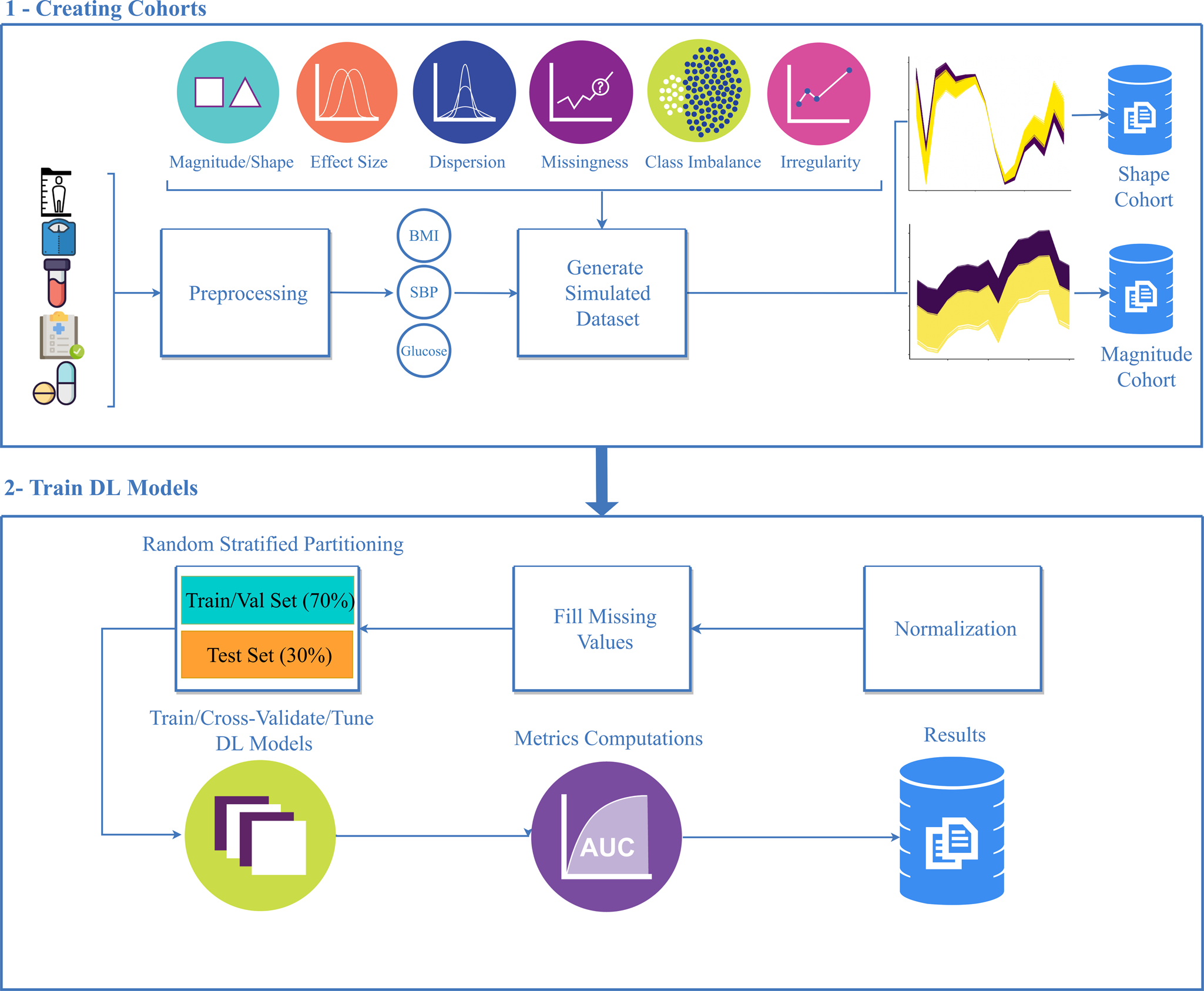
Figure 1.1 Simulation study workflow.
① Longitudinal electronic health record (EHR) data were collected from six randomly selected patients and used to generate reference body mass index (BMI) trajectories using weight and height measurements. Magnitude and shape simulation cohorts were generated from the reference trajectories.
② Simulation cohorts are used to train deep learning models after Z-score normalization, missing value imputation, and partitioning data into training/test sets. Cohorts were randomly partitioned to have training/validation, and test sets of 70%, and 30% respectively.
2.1.1.1.2. Step 2: assess the performance of the most effective DL model on actual EHR data for the prediction of pediatric type-2 diabetes (T2D).
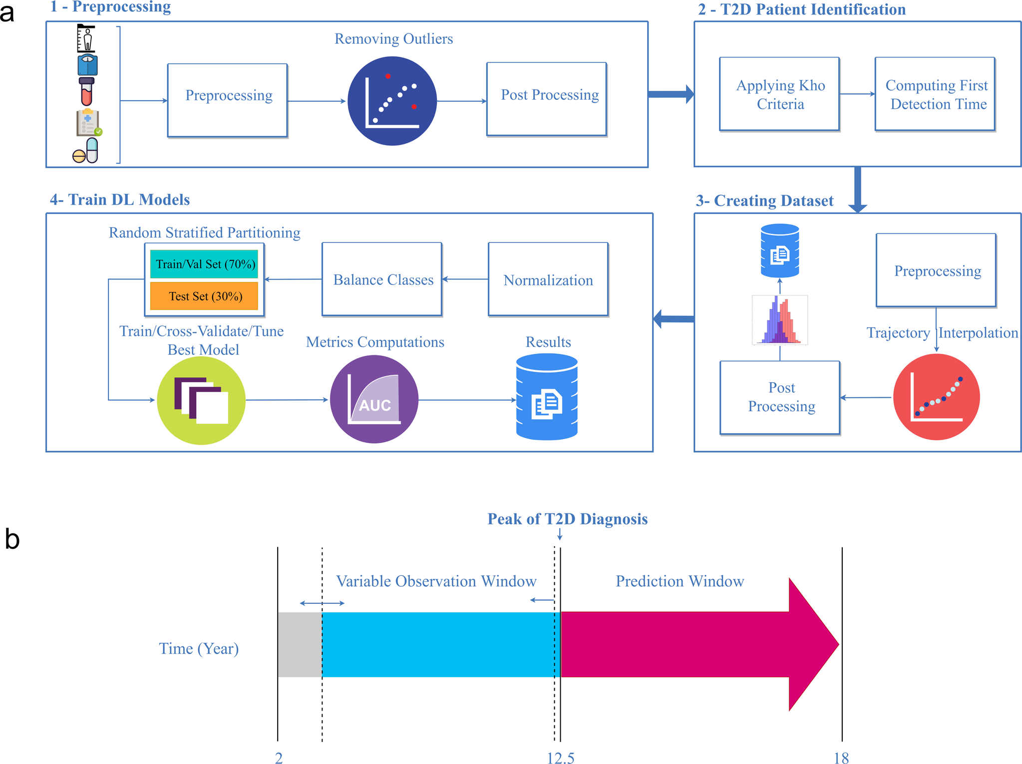
Figure 1.2 Modeling real-world pediatric type-2 diabetes (T2D) workflow.
a:① Longitudinal weight and height data were extracted from the EHR. Height and weight outliers were removed and patients with <2 BMI records were excluded.
② Patients were labeled as underweight, normal weight, overweight, obese, and severe-obese according to the Centers for Disease Control criteria, and were classified as those that developed T2D or did not develop T2D.
③ Trajectories were then harmonized such that each trajectory consisted of a single BMI record per year.
④ Subsequent modeling steps were consistent with those shown in ② of Figure 1.1
b Depicts the observation and prediction window definitions. The observation window varied from 2 years old to the average age of T2D in pediatric patients (12.5 years old), and the prediction window was fixed from 13 to 18 years old.
2.1.1.2. Metrics
| ROC Curve | a graphical representation of a model's performance. It plots the True Positive Rate (Sensitivity) against the False Positive Rate (1 - Specificity) at various classification thresholds. |
| AUC ↑ | the area under the ROC curve. It quantifies the overall ability of the model to discriminate between the two classes. A perfect model achieves an AUC of 1, while a random or poor model would have an AUC of 0.5. |
| FDR P values of the DeLong's test |
DeLong's test is typically used to compare the performance of two or more classification models, and the FDR-adjusted p-values are employed to control the error rate associated with multiple comparisons. If the FDR P-value is less than a certain threshold (usually 0.05), it indicates that the performance differences between the models in multiple comparisons are statistically significant. |
2.1.1.3. Results
2.1.1.3.1. Model performance on simulated data
①Data missingness

Figure 1.3 Area under the receiver operating characteristic curve (AUC) differences of train and test sets over different levels of missingness
GAF-CNN was robust over various degrees of missingness with AUCs of 0.93, 0.92, 0.90, and 0.83 for missingness of 0%, 10%, 25%, and 50%, respectively. TSF-CNN performed comparably with AUCs ranging from 0.93 0.91, 0.89, and 0.81 for 0%, 10%, 25%, and 50% missingness. Models that were the most detrimentally impacted by missingness were Transformer, MLP, and ResNet with respective AUCs of 0.52, 0.55, and 0.59 at 50% missingness.
**Multilayer perceptron (MLP); Fully convolutional neural network (FCNN); Time series forest MLP (TSF-MLP); Time series forest CNN (TSF-CNN); Gramian angular field CNN (GAF-CNN); Residual network (ResNet); Recurrent neural network—fully convolutional network (RNN-FCN); Convolutional-recurrent neural network (C-RNN)
②Overall accuracy

Figure 1.4 Critical difference plot to compare the model’s performance based on their test AUC (Lower CD value is better).
Overall model accuracy was determined using a Friedman test to evaluate model AUCs. TSF-CNN was ranked as the best model but was not statistically significantly better than GAF-CNN, which was ranked second (P > 0.05). These models were followed by CRNN, LSTM-FNC, FCNN, TSF-MLP, MLP, ResNet, and Transformer, respectively, and these were all statistically significantly different from each other (P < 0.05)
③Model overfitting

Figure 1.4 Model overfitting was evaluated by comparing the AUC differences for each deep learning method in the training sets and the test sets based on (c) changes in trajectory magnitude and (d) changes in trajectory shape.
All DL models demonstrated similar accuracies between the training and test sets in the magnitude cohorts (AUCs ~0.92). The difference in AUCs between the test and training sets was negligible with the highest difference observed with ResNet, which had a mean AUC difference of 0.0015. More substantial model overfitting was observed in the shape cohort. TSF-CNN demonstrated the least model overfitting with a difference in AUC of 0.0051, and RNN-FCN demonstrated the greatest model overfitting with a difference in AUCs between training and test cohorts of 0.0227.
2.1.1.3.2. Performance of the TSF-CNN model to predict pediatric type-2 diabetes (T2D) in a real-world cohort.
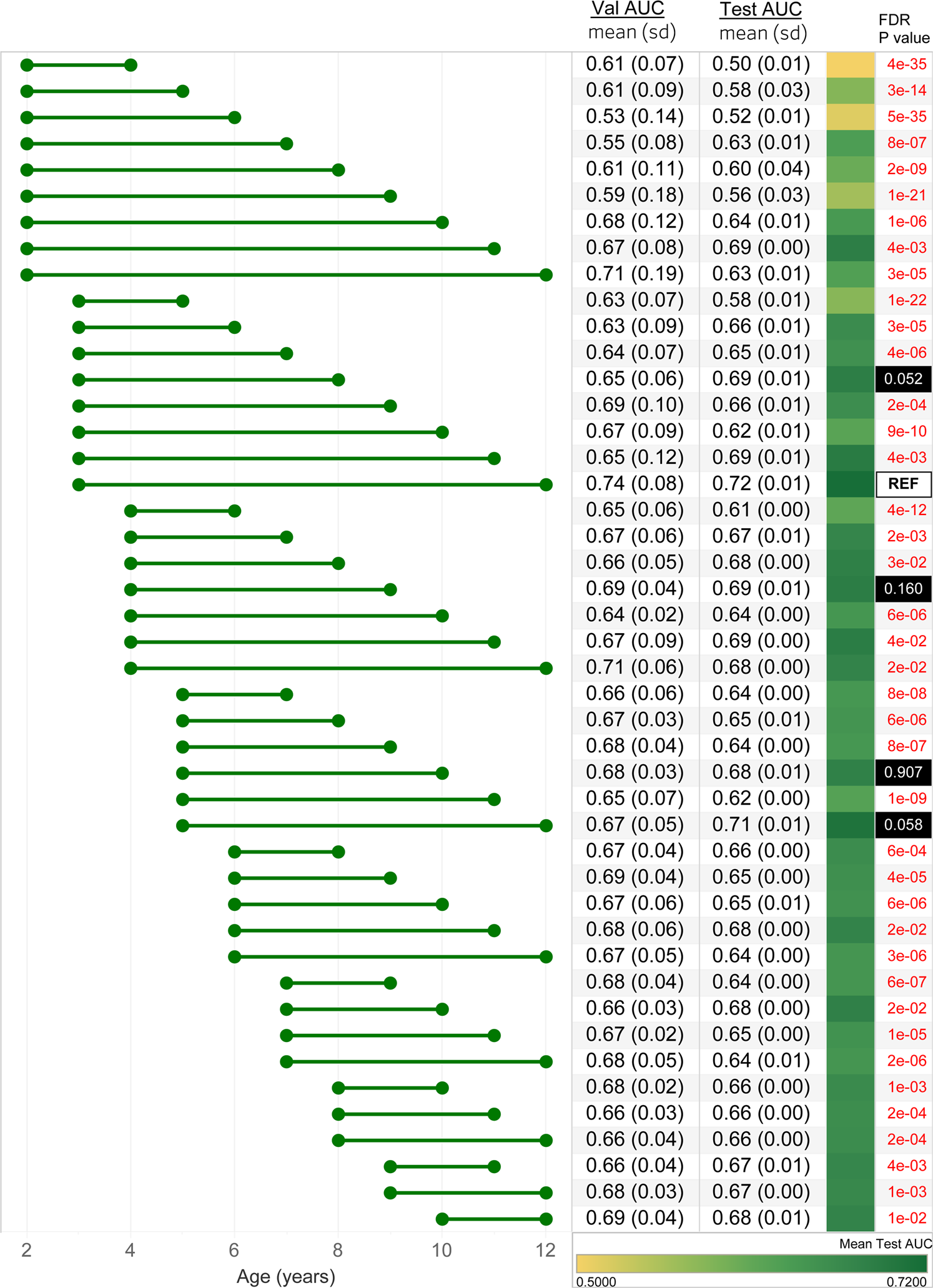
Figure 1.5 Performance of the TSF-CNN model
In general, model performance improved when the observation window included a wider range of ages, and the max-age was closer to the maximum of 12 years old. The model with the observation windows spanning 3–12 years had the highest accuracy (AUC = 0.72). However, models constructed on ages 5–12 (AUC = 0.71), 3–8 (AUC = 0.69), 4–9 (AUC = 0.69), 5–10 (AUC = 0.68) were not statistically different from the best performing model (FDR P < 0.05). Models incorporating fewer and younger ages performed worse with the observation window spanning 2-4 demonstrating the lowest accuracy (AUC = 0.50)
Different age ranges incorporated in the model are shown with the horizontal bars. The mean and standard deviation of cross-validation (Val) AUCs and test AUCs are shown.
The third column represents the model area under the receiver operating characteristic curve (AUC when it is applied to the withheld test set) with a green gradient indicating the accuracy of the prediction.
The fourth column indicates the FDR P values of Delong’s test for each AUC compared to the best-performing age range, ages 3–12, annotated with “REF”. Models with a FDR P < 0.05 are shown in red.
2.1.1.4. Conclusion
In cases of significant data missingness, GAF-CNN exhibited the highest prediction accuracies among the models, achieving AUCs of 0.90 and 0.83 with 25% and 50% missing data, respectively. While the GAF-CNN approach outperformed others for shape simulation, TSF-CNN closely followed suit, and their AUCs were statistically equivalent across all simulated scenarios (P > 0.05).
These findings identify TSF-CNN and GAF-CNN as promising frameworks for leveraging longitudinal clinical measurements in predictive modeling, as demonstrated through the prediction of T2D onset using longitudinal BMI trajectories from pediatric patients.
TSF-CNN is built upon the framework of time series forests, which enables efficient feature extraction and classification tasks on time series data. On the other hand, GAF-CNN leverages the Gramian Angular Field technique to transform time series data into an image-based representation, facilitating a better understanding and processing of the data by deep learning models. As a result, both frameworks possess the capability to handle time series data, making them suitable for the analysis of long-term clinical measurement data in the medical field.
2.1.2. Deep Framework for Physician Burnout Prediction Using Activity Logs in Electronic Health Records[3]
2.1.2.1. Longitudinal Medical Data
Electronic Health Record (EHR) activity logs represent documentation of a clinician's interactions with the EHR system, encompassing a detailed record of all actions undertaken within the system, including timestamps, patient information, specific activities performed, and user identification, providing a comprehensive account of a clinician's professional activities.
Burnout Surveys: intern and resident physicians who were part of various clinical rotations (such as Internal Medicine, Pediatrics, and Anesthesiology), each lasting 4 weeks, participated in surveys designed to assess their recent well-being status. These surveys were administered at 4-week intervals, aligning with the conclusion of each rotation period.
2.1.2.2. Main Challenges
① The initial hurdle lies in the extraction of valuable insights from unstructured raw log files, which capture information about more than 1,900 categories of actions within Electronic Health Records (EHR). These actions encompass activities such as reviewing reports, notes, laboratory tests, order management, and the documentation of patient care activities.
②The subsequent challenge in developing a deep predictive model for burnout revolves around dealing with the extensive volume of activity logs, characterized by lengthy data sequences, and the scarcity of labels, as there are relatively few responses available from burnout surveys.
③ An ideal predictive model should effectively capture and utilize the hierarchical structure present in physician activity logs, which reflect the multi-layered nature of clinical work activities and their varying temporal patterns.
2.1.2.3. Temporal models

Figure 1.6 An overview of Hierarchical burnoutPrediction based on activity logs (HiPAL) framework
This includes a pre-trained time-dependent activity embedding mechanism specifically designed for activity logs, a hierarchical predictive model capable of capturing physician behaviors across multiple temporal levels, and a semi-supervised framework that leverages knowledge from unlabeled data. Importantly, the HiPAL framework is adaptable and can be built upon any convolution-based sequence model as its foundational base model.
2.1.2.4. Results
2.1.2.4.1. Metrics
| AUROC (Area Under the Receiver Operating Characteristic Curve) ↑ | assess the overall performance of a classification model. It evaluates the ability of a model to distinguish between positive and negative classes by plotting the True Positive Rate (TPR) against the False Positive Rate (FPR) across different classification thresholds |
| AUPRC (Area Under the Precision-Recall Curve) ↑ | measures a classification model's precision and recall trade-off. It is particularly useful when dealing with imbalanced datasets, where one class significantly outnumbers the other. A higher AUPRC score reflects better model performance, especially in cases where positive class detection is crucial. |
2.1.2.4.2. Results

Table 1.1 Random repeated cross-validation results
a comprehensive performance summary of various models, encompassing non-deep learning models, single-level sequence models, hierarchical models, and semi-supervised models.
- GBM/SVM/RF: Gradient Boosting Machines implemented withXGBoost, Support Vector Machines, and Random Forests,
- FCN: Full Convolutional Networks,
- CausalNet: A primitive architecture of TCN with fixed dilation and Max Pooling layers used for videos
- ResTCN. A popular TCN architecture with exponentially enlarged dilation. The cross-layer residual connections enable the construction of a much deeper network.
- H-RNN: Hierarchical RNN, a multi-level LSTM model used for long video classification.
- HierGRU: Hierarchical baselines, implemented with GRU as the HiPAL low-level encoder.
- Semi-ResTCN: A semi-supervised single-level model baseline, Implemented with ResTCN. We pre-train the single-level TCN with an TCN-AE.
- As variants of the proposed hierarchical framework, HiPAL-f, HiPAL-c, and HiPAL-r corresponds to the HiPAL-based predictive model with the low-level encoder Φ instantiated by FCN, CausalNet, and ResTCN.
2.1.2.5. Conclusion
In a broader context, the non-deep learning models, specifically GBM (Gradient Boosting Machine), SVM (Support Vector Machine), and RF (Random Forest), exhibit lower predictive performance when compared to deep learning models. This discrepancy could arise from the limited effectiveness of basic statistical features, such as EHR timestamps and the count of reviewed notes, in capturing intricate activity patterns and temporal dependencies.
When contrasted with the supervised HiPAL models, it is evident that, on average, all three Semi-HiPAL counterparts exhibit superior performance (except for Semi-HiPAL-r, which shows a slightly inferior AUPRC compared to HiPAL-r). This observation highlights the capability of the semi-supervised framework, facilitated by pre-training, in effectively deriving generalizable patterns from unlabeled activity logs and subsequently transferring this knowledge to HiPAL. This insight suggests the potential for enhanced prediction efficacy in real-world clinical scenarios, particularly when the availability of costly burnout labels is limited, while there exists a substantial volume of unlabeled activity logs.
Within the HiPAL framework, a specialized time-dependent activity embedding mechanism is incorporated, designed to process and encode raw data directly from the Electronic Health Record (EHR) activity logs. Non-temporal models, lacking the ability to handle temporal information, are ill-equipped to effectively predict physician burnout.
2.2. Omics and Molecular Data
2.2.1. Longitudinal microbiome data [4]
2.2.1.1. Longitudinal microbiome data
The temporal alterations within the microbiome can capture a wealth of information beyond what is achievable through single-point inference, due to their ability to encapsulate dynamic patterns.
The PROTECT study comprises 428 participants diagnosed with new-onset pediatric ulcerative colitis in the United States and Canada, and the study spanned one year. Stool samples from these subjects were subjected to 16s rRNA gene amplicon sequencing using the Illumina MiSeq Platform.
the DIABIMMUNE study focuses on investigating the influence of hygiene on the development of Type 1 Diabetes and other autoimmune diseases. It involved the collection of three years' worth of monthly stool samples, laboratory assays, and comprehensive questionnaires. A total of 1584 stool samples from this study were subjected to 16s rRNA gene amplicon sequencing using the Illumina HiSeq 2500 Platform.
2.2.1.2. Challenges
① The presence of missing information across different time points for various subjects, resulting in an uneven distribution of microbiome data.
② A large number of operational taxonomic units (OTUs) in microbiome profiles but a limited number of subjects at each time point.
2.2.1.3. Temporal models

Figure 2.1 Architecture of CNN-LSTM.
(a) The first self-distillation method consists of several sub-classifiers to predict the labels of the ground truth and the prediction of the main classifier
(b) The second self-distillation method uses the model’s previous epoch prediction as a regularization
2.2.1.4. Metrics & Evaluation
2.2.1.4.1. Metrics
| AUC ↑ | A higher AUC indicates better model performance, with a perfect classifier having an AUC of 1. |
| F1 Score ↑ | combines precision and recall to evaluate the performance of a binary classification model. It is the harmonic mean of precision and recall and provides a balance between these two metrics. |
2.2.1.4.2. Results
① Prediction performance based on the PROTECT study

PCA, principal component analysis; stdev, standard deviation.
Bolded texts are the highest performance.
Table 2.1 Prediction performance of the 10-fold cross-validation on the PROTECT study without self-distillation
② Prediction based on the DIABIMMUNE study

Bolded texts are the highest performance.
Table 2.2 Prediction performance of the 10-fold cross-validation on the DIABIMMUNE study without self-distillation
2.2.1.5. Conclusion [4]
Deep learning techniques have demonstrated the ability to classify disease severity and allergic reactions by leveraging longitudinal gut microbiome data. By considering the temporal dynamics of the gut microbiome, models can extract richer feature representations, enabling the classification of disease severity in the PROTECT study and allergic reactions in the DIABIMMUNE study. The integration of Convolutional Neural Networks (CNN) with Long Short-Term Memory (LSTM) models has been instrumental in enhancing model performance, leading to higher AUC scores, as observed in both the PROTECT and DIABIMMUNE studies.
2.2.2. Principles and challenges of modeling temporal and spatial omics data [5]
An overview paper
2.2.2.1. Conclusion
Research endeavors featuring temporal or spatial resolutions are indispensable for comprehending the molecular dynamics and spatial interdependencies that underlie biological processes or systems.
Within the domain of precision health, the utilization of longitudinal (multi)omic profiling is regarded as a means to monitor a group of patients throughout their treatment journey or for the prospective characterization of health conditions across the entire span of an individual's life.
Sequence data can be modeled with RNNs, for example, to predict the stability, subcellular localization, or homology of proteins or to impute missing methylation states in single-cell data.
2.3. Patient-generated data
2.3.1. IoT Sensors Empowered [6]
Intelligent medical devices and wearable technologies play a significant role within the Internet of Things (IoT) ecosystem, as they have the capacity to gather diverse sets of patient-generated health data over time and offer preliminary diagnostic insights.
An intracranial hematoma (ICH) is a clot in the brain that forms beneath the skull.
2.3.1.1. Longitudinal Medical Data
PSG polysomnography measurements (ECG & EEG), blood pressure, and airflow are all recorded together with the date and time by IoT devices,
2.3.1.2. Proposed Work System
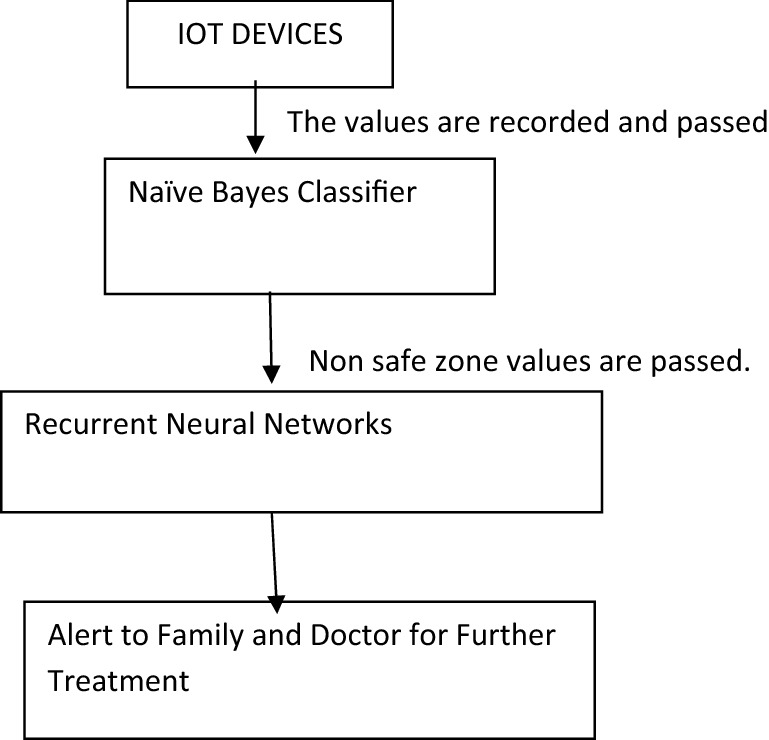
Figure 3.1 Block diagram of the proposed system
Blood flow, blood pressure, and airflow measurements are linked to an Arduino board equipped with a WiFi module, which transmits data to a Naive Bayes Classifier.
This Naive Bayes Algorithm categorizes sensor data into two groups: safe and non-safe.
In cases where individuals fall into the non-safe category, intracranial images are captured and transmitted to recurrent neural networks.
These recurrent neural networks are employed to predict patients at risk of hemorrhage, and immediate notifications are dispatched to healthcare professionals or the patient's family, prompting necessary actions.
Patients without hemorrhage are regularly monitored, with values assessed on a routine basis.
2.3.1.3. Results
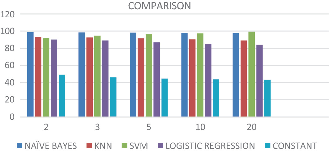
Figure 3.2 Naïve Bayes and RNN comparison with all other algorithms
2.3.1.4. Conclusion
Recurrent Neural Networks (RNNs) predict patients with hemorrhages and communicate this information to both the patient's family and the doctor via a WiFi-enabled Arduino board. The RNNs achieve an impressive overall accuracy rate of 97%. When Naïve Bayes is combined with RNN, it consistently outperforms other machine learning algorithms in terms of accuracy, making it the most reliable choice for predicting hemorrhage patients.
The Internet of Things (IoT) gathers a vast amount of data with temporal information, and temporal models such as Recurrent Neural Networks (RNNs) excel at effectively processing this time-sensitive data.
2.3.2. From Social Media [7]
2.3.2.1. Longitudinal Medical Data
By tracking users for nearly three months, about 200 tweets, individuals with depression were identified from a dataset of COVID–19–related tweets by detecting signals such as self-descriptions as "depression fighters" and specific phrases related to depression in tweets and profile descriptions.
Conversely, individuals who were not considered to have depression were randomly selected from Twitter users who did not exhibit depression-related terms in their recent tweets or profile descriptions, serving as the control group.
2.3.2.2. Goal
The hypothesis was that subtle linguistic differences existed between the depression and nondepression groups. The goal is to develop a model capable of effectively discerning these linguistic nuances for accurate user classification.
2.3.2.3. Metrics & Evaluation
2.3.2.3.1. Metrics
| Accuracy | measures the proportion of correctly classified samples by a model out of the total number of samples. It is used to assess the overall performance of a model. |
| F1 Score | a weighted average of precision and recall, designed to balance a model's precision and recall, especially suitable for imbalanced datasets. |
| AUC | It represents the area under the curve formed by the true positive rate and the false positive rate at various thresholds, measuring a model's classification capability. |
| Precision | measures the proportion of correctly predicted positive samples by a model out of all samples predicted as positive. It is used to assess the model's accuracy. |
| Recall | measures the proportion of correctly predicted positive samples by a model out of all actual positive samples. It is used to assess the model's comprehensiveness or ability to identify all positive instances. |
2.3.2.3.2. Results
chunk-level performance

Figure 3.3 Chunk-level performance (%) of all 5 models on the 500-user testing set using training-validation sets of different sizes.a
: We used 0.5 as the threshold when calculating the scores.
b: AUC: area under the receiver operating characteristic curve.
c: BiLSTM: bidirectional long short-term memory.
d: CNN: convolutional neural network.
e: BERT: Bidirectional Encoder Representations from Transformers.
f: RoBERTa: Robustly Optimized BiLSTM Pretraining Approach.
g: Italics indicate the best-performing model in each column.
2.3.2.4. Conclusion
An initial observation revealed that irrespective of the model type employed, the classification performance demonstrated enhancement with the expansion of our train-validation set. This underscores the critical importance of obtaining a substantial volume of training data when constructing depression classification models.
Social media platforms such as Twitter serve as a valuable resource, furnishing copious amounts of data for this purpose. For data like tweets, which may not exhibit as tight temporal correlations, temporal models may not demonstrate their distinctive advantages as prominently.
2.4. Imaging Data
2.4.1. CT: lung cancer [8]
2.4.1.1. Longitudinal Medical Data
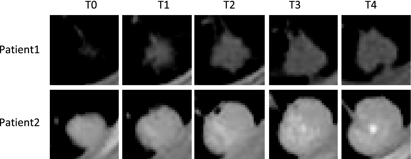
Figure 4.1 CT imaging data of the same pulmonary nodules in two patients at five different stages
2.4.1.2. Main problems in computer-aided diagnosis (CAD) and survival prediction of lung cancer
① Conventional methods for predicting the survival of lung cancer patients are mainly based on tumor stage
② Most of the existing CAD methods for lung lesions are studied for images of a single period, ignoring the impact of the progressive evolution of lesion characteristics on survival and not consider the correlation between multi-period computed tomography (CT) images.
③ Multiple types of medical data are not yet integrated or insufficiently integrated.
2.4.1.3. Temporal models
2.4.1.3.1. MS-ResNet structure
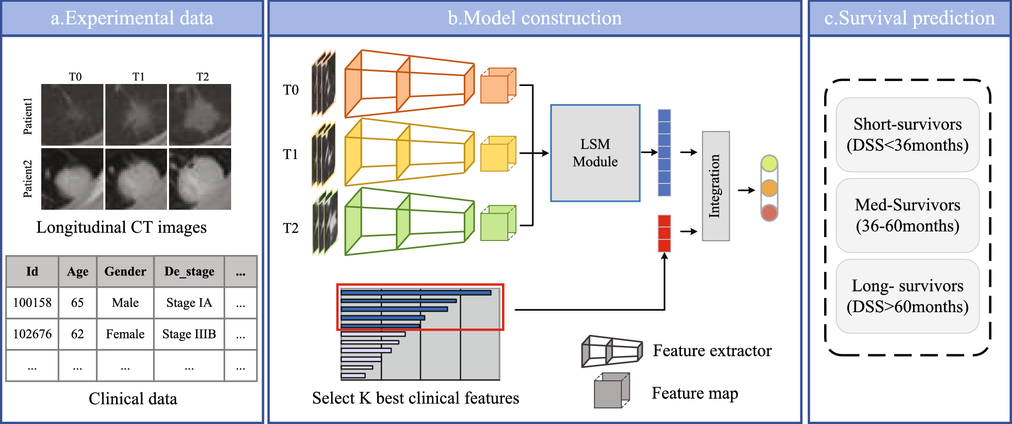
Figure 4.2 The structure of ,S-ResNet
a: experimental data: information on 198 patients from the National Lung Screening Trial (NLST) dataset, and each patient data includes follow-up CT image data and clinical record data for 3 periods
b: model construction: extracting deep features of CT images (3-branch residual network), capturing temporal information(longitudinal self-attention mechanism module), integrating deep features and clinical attributes(describe participants, e.g. smoking and alcohol use, disease diagnosis, family genetic history, follow-up records, etc. and then select K best clinical attributes)
c: survival prediction: results will be classified as short survivor, medium survivor, and long survivor
2.4.1.3.2. Spatiotemporal attention module
Images from different periods contain different characteristics. a longitudinal self-attention mechanism (LSM), which can capture the rich global spatial–temporal relationships between pixels in the whole space-time, to obtain more discriminative features.
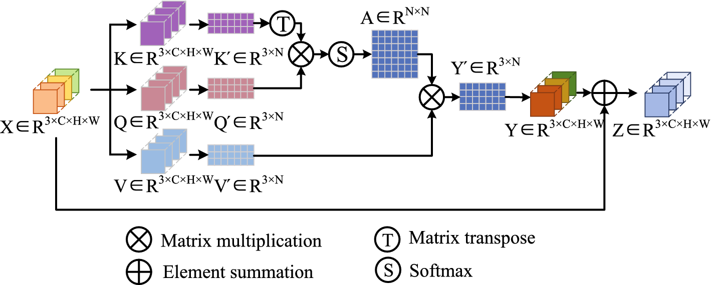
Figure 4.3 Longitudinal self-attention mechanism (LSM)
2.4.1.4. Metrics & Evaluation
2.4.1.4.1. Metrics
① DSS prediction performance: estimation of a patient's likelihood of surviving a particular disease based on relevant patient data and disease-specific characteristics.
The samples are divided into long-survival (greater than 60 months) med-survival (between 36 and 60 months), and short-survival (less than 36 months) patients according to the thresholds. They employ Accuracy, macroF1, and microF1 to evaluate the classification performance of DSS survival for lung cancer patients.
| Accuracy |
measure the overall correctness of a classification model Accuracy = (Number of Correct Predictions) / (Total Number of Predictions) |
| Macro F1-Score |
balance precision and recall MacroF1 = (F1-Score_Class_1 + F1-Score_Class_2 + ... + F1-Score_Class_n) / n where n is the number of classes. |
| Micro F1-Score |
evaluate the overall performance of a classification model, giving equal importance to each prediction MicroF1 = 2 * (Precision * Recall) / (Precision + Recall) |
② Confusion matrix: visualize the performance of a classification model by comparing predicted and actual class labels
2.4.1.4.2. Results
① The classification of the three categories is performed correctly.
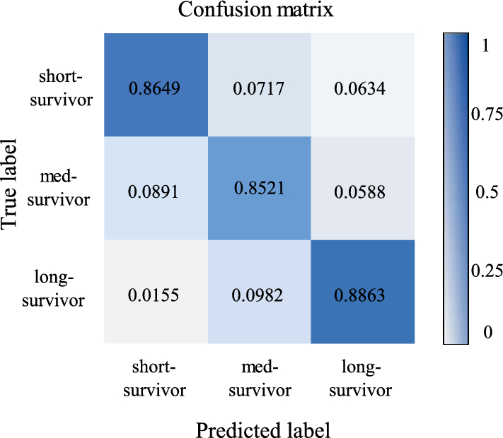
Figure 4.4 Condusion materix
The long-survivor has the highest percentage of correct predictions with 88.63%, followed by the short-survivor with 86.49%, and finally the med-survivor with 85.21%.
② Ablation experiment: to see if the modification of the model works

Table 4.1 Comparison of accuracy resulting from various fusion approaches
The initial three rows: the use of ResNet solely with images from time periods T0, T1, and T2; (Single image)
"mean" row: the average classification accuracy across these three periods.
MR-Net: multi-branch ResNet, which simultaneously takes images from all three periods as inputs, integrating multiple deep features directly for prediction.
MR-Net + LSM: incorporate a longitudinal self-attention mechanism module
MS-ResNet: encompasses MR-Net with the LSM module and further integrates filtered clinical attributes for prediction.
③ Comparison with other models

Table 4.2 Comparison of the methodology and performance of our proposed model with the state-of-the-art studies
MS-ResNet is better than other models
2.4.1.5. Conclusion
① To assess the impact of integrating multi-period CT image data on Disease-Specific Survival (DSS) prediction, the author compared MS-ResNet performance against one that relied solely on single-period CT data (ResNet). Table 4.1 presents compelling evidence supporting the efficacy of survival classification when leveraging temporal information inherent in multi-phase CT images. This underscores the necessity of considering multi-temporal information (MTI) in similar medical diagnostic applications.
Directly integrating the deep features from the three periods via MR-Net leads to a moderate improvement in classification accuracy, although the effect is not particularly pronounced.
The incorporation of the LSM (Long Short Memory) module into the fusion network allows for the allocation of appropriate weights to features from different periods, resulting in a notable enhancement in prediction accuracy.
② A comprehensive comparative analysis with existing studies in a similar domain, as outlined in Table 4.2, MS-ResNet outperforms others in multiple metrics, enabling precise classification of lung cancer patients with an accuracy rate of 86.78%. These results underscore the essential role and practical viability of integrating longitudinal data with clinical information in research, emphasizing the profound significance of Disease-Specific Survival (DSS) prediction.
2.4.2. MRI [10]
2.4.2.1. Longitudinal Medical Data [9]

Figure 4.5 Longitudinal axial brain MRI slices of a mild cognitive impairment patient from the ADNI dataset
2.4.2.2. Main problems:
Alzheimer's disease (AD) stands as a significant health challenge in developed nations, early intervention can notably delay the need for institutional care and prolong patient independence. Recent studies have explored the use of two-dimensional (2D) CNNs applied to magnetic resonance imaging (MRI) scans for AD detection. To adapt 2D CNNs for the analysis of three-dimensional (3D) MRI volumes, each MRI scan is partitioned into 2D image slices.
While 2D CNNs are effective at capturing spatial relationships within individual image slices, they lack the ability to capture temporal dependencies among the 2D image slices within a 3D MRI volume. This research addresses this limitation by introducing deep sequence-based networks to model the sequence of MRI features generated by the CNN, specifically for the purpose of Alzheimer's Disease (AD) detection.
2.4.2.3. Temporal models
2.4.2.3.1. CNN and RNN

Figure 4.6 A block diagram of our AD detection system involving the CNN and RNN models.
Firstly, use ImageNet, a dataset of 1000 object categories, to initialise the 2D CNN model ( cannot capture the spatial information of 3D MRIs), The trained 2D CNN can be used for feature extraction
Secondly, the RNN is for understanding the relationship between the sequence of extracted features corresponding to MRI image slices.
However, TCNs can simultaneously perform feature extraction and classification within the same sequence-based task, addressing the independence issue between the feature extraction step in CNN and the classification step in RNN.
2.4.2.3.2. The TCN model

Figure 4.7 (a) Stacked convolutional layers in TCNs, (b) a residual block.
The core building blocks of a TCN are dilated causal convolutional layers that run over time steps of a sequence.
Causal convolutions ensure that a filter at time step 't' only has access to inputs preceding time 't,' thereby preventing information leakage from the future to the past, similar to LSTM and GRU structures. To capture information from previous time steps, multiple convolutional layers are stacked on top of each other. The dilation factor 'd' within these convolutional layers governs the size of the receptive field, potentially enabling an exponentially large receptive field. The receptive field denotes the segment of sequential time steps that can activate neural responses.
A general TCN model comprises several residual blocks, each of which combines two dilated causal convolution layers with identical dilation factors, followed by normalization, ReLU activation, and dropout layers.
2.4.2.4. Metrics & Evaluation
2.4.2.4.1. Metrics
| Accuracy | the percentage of correctly classified test subjects |
| Sensitivity | the percentage of evaluated test subjects suffering from AD who were correctly classified as such |
| Specificity | the percentage of evaluated healthy test subjects correctly classified as healthy |
2.4.2.4.2. Results
① Ablation experiment: to see if the modification of the model works

Table 4.3 Accuracies of the proposed sequence-based deep models on the selected dataset (AD vs. NC).
Approach 1 leveraged pre-trained CNN models to extract features, which were subsequently fed into a TCN, maintaining spatial relationships;
Approach 2 directly employed original 79×79 greyscale coronal images as inputs to a TCN for simultaneous feature extraction and classification, although filters were initialized randomly
LSTM, BiLSTM, and GRU models are revised versions of RNNs with more complex structures, including gates.
In the cases of ResNet-18 + LSTM, ResNet-18 + BiLSTM, ResNet-18 + GRU, and ResNet-18 + TCN, the overarching strategy was to incorporate a sequence-based model alongside ResNet-18 to enhance the accuracy of Alzheimer's Disease (AD) detection.
② A summary of the implemented input data management methods for AD detection.
| Methods | Strengths | Limitations |
|---|---|---|
| Sequence-based |
⁃ Prevents facing millions of parameters during training and provides more simplified networks ⁃ Can benefit from transfer learning using 2D datasets
|
⁃ Feature extraction and classification are not performed simultaneously ⁃ Cannot benefit from transfer learning using 2D datasets |
a: Only 2D CNN + RNN and 2D CNN + TCN; b: Only TCN Approach 2.
2.4.2.5. Conclusion
For Table 4.3, gates play a pivotal role in controlling the information flow within the sequential chain, allowing for the removal or incorporation of historical data into the network.
LSTM cells update their parameters based on past images in a sequence, preserving only past information.
BiLSTM cells update parameters based on both past and future images in a sequence, capturing information from both directions.
GRU cells have a structure similar to LSTM but with simpler architecture and faster training, controlling information flow in a comparable manner to LSTM.
Among the evaluated RNN configurations, ResNet-18 + LSTM demonstrated the most favorable performance in AD detection, achieving an accuracy of 84%, a sensitivity of 80%, and a specificity of 88%. And, the original ResNet 18 cannot consider the temporal information. This suggests that when combining LSTM and ResNet, such a model can effectively handle temporal information, leading to improved performance.
In contrast, TCNs offer practicality by dispensing with the necessity of a feature extraction interface, allowing them to directly extract features from MRI coronal slices while simultaneously capturing their interrelationships. As demonstrated in Table 4.3, sequence-based models exhibit enhanced accuracy in AD detection. Specifically, TCN with 4 residual blocks in Approach 2, ResNet-18 + TCN with 3 residual blocks in Approach 1, and ResNet-18 + LSTM outperformed ResNet-18 in terms of accuracy. Nonetheless, the outcomes for ResNet-18 + BiLSTM revealed that introducing a sequence-based network for independently extracted features occasionally introduced ambiguities into the sequence-based classification.
When comparing Approaches 1 and 2, Approach 2, which involves direct feature extraction and classification by the TCN, demonstrated superior accuracy in AD detection. This unique attribute of TCNs conferred an advantage over RNNs for image-based tasks.
3. Conclusion
3.1. Medicine
Interdisciplinary advances have played a pivotal role in advancing medicine, not only diversifying longitudinal medical data but also simplifying its acquisition.
Fundamental research in biology and molecular biology has laid the groundwork for a profound understanding of life processes and disease mechanisms. The evolution of molecular biology has enabled in-depth insights into biology at the genetic, protein, and cellular levels, forming the foundation for precision medicine and gene therapy.
Innovations in engineering disciplines, such as computer science and physics, have supported the development of medical devices, imaging technologies, and healthcare information systems, acquiring longitudinal medical data more accessible and contributing to the diagnosis, monitoring, and treatment of medical conditions.
The proliferation of the Internet of Things (IoT) has facilitated the convenient collection of longitudinal medical data from patients, allowing real-time monitoring and the capture of relevant patient information.
Cross-disciplinary research has fostered collaboration and synergy among various fields, leading to novel approaches and solutions in medicine. These interdisciplinary efforts have been instrumental in advancing our understanding of longitudinal medical data and its applications in healthcare.
3.2. Longitudinal Medical Data & Temporal Models
The temporal aspect in longitudinal data allows for the tracking of changes and developments over time, providing valuable insights into medical conditions and patient outcomes.
In contrast, non-longitudinal medical data lacks this time-dependent perspective, often providing a static snapshot of a single point in time.
The incorporation of temporal models in the analysis of longitudinal medical data enables the modeling of temporal dependencies and patterns, enhancing our ability to predict, understand, and manage medical conditions more effectively compared to non-temporal models that do not account for the dynamic nature of such data.
3.3. Precision Medicine
The integration of longitudinal medical data, temporal models, and multidisciplinary collaboration holds the potential to propel the advancement of precision medicine, offering substantial benefits to patients.
This convergence allows for a comprehensive understanding of a patient's health journey over time, enabling tailored interventions, early disease detection, and personalized treatment strategies.
The synergy between longitudinal data and temporal models empowers healthcare professionals with the tools to make more informed decisions and deliver targeted care, ultimately improving patient outcomes and enhancing the overall healthcare experience.
4. Reference
[1] Sarwar T, Seifollahi S, Chan J, et al. The secondary use of electronic health records for data mining: Data characteristics and challenges[J]. ACM Computing Surveys (CSUR), 2022, 55(2): 1-40.
[2] Javidi H, Mariam A, Khademi G, et al. Identification of robust deep neural network models of longitudinal clinical measurements[J]. NPJ Digital Medicine, 2022, 5(1): 106.
[3] Liu H, Lou S S, Warner B C, et al. HiPAL: A Deep Framework for Physician Burnout Prediction Using Activity Logs in Electronic Health Records[C]//Proceedings of the 28th ACM SIGKDD Conference on Knowledge Discovery and Data Mining. 2022: 3377-3387.
[4] Fung D L X, Li X, Leung C K, et al. A self-knowledge distillation-driven CNN-LSTM model for predicting disease outcomes using longitudinal microbiome data[J]. Bioinformatics Advances, 2023, 3(1): vbad059.
[5] Velten B, Stegle O. Principles and challenges of modeling temporal and spatial omics data[J]. Nature Methods, 2023, 20(10): 1462-1474.
[6] Theodore S K A, Selvakumar K, Revathy G. Brain Depletion Recognition Through Iot Sensors Empowered with Computational Intelligence[C]//Futuristic Trends in Networks and Computing Technologies: Select Proceedings of Fourth International Conference on FTNCT 2021. Singapore: Springer Nature Singapore, 2022: 295-302.
[7] Zhang Y, Lyu H, Liu Y, et al. Monitoring depression trends on Twitter during the COVID-19 pandemic: observational study[J]. JMIR infodemiology, 2021, 1(1): e26769.
[8] Han J, Xiao N, Yang W, et al. MS-ResNet: disease-specific survival prediction using longitudinal CT images and clinical data[J]. International Journal of Computer Assisted Radiology and Surgery, 2022, 17(6): 1049-1057
[9] Kim S T, Küçükaslan U, Navab N. Longitudinal brain MR image modeling using personalized memory for Alzheimer’s disease[J]. IEEE Access, 2021, 9: 143212-143221
[10] Ebrahimi A, Luo S, Chiong R, et al. Deep sequence modelling for Alzheimer's disease detection using MRI[J]. Computers in Biology and Medicine, 2021, 134: 104537.