1. What is adversarial example?
Adversarial examples are inputs that are intentionally crafted/attacked by an adversary to fool a model to make a mistake. These examples are generally indistinguishable from the original self to the humans or an oracle. They have several characteristics:
- Generally within L-p<ξ norm of base example(1)
- Since we don't have a clear description of human perception, correct p and ξ values are unknown(1)
- Most of the literature uses L-1, L-2 and L-infinity norms
- Can be constructed in many ways
- Optimize for only one example (L-p bounded adversarial examples)
- Optimize for multiple examples (Universal Adversarial Perturbations)
- Different optimization methods possible
- Can be white-box or black-box(1)
Name Uses Trivial? White-Box Model and/or gradients 
Black-Box Only outputs of model 
- Can be targeted or untargeted(1)
- Targeted
- Attacker has a specific class to be misclassified as (Duck → Horse)
- Untargeted
- Attacker just wants an example to be misclassified, regardless as resulting classification (Duck → Not Duck)
- Targeted
- Why indistinguishable to humans?
- On a cat/dog classifier, you can turn a cat image to a dog image with enough perturbation. This wouldn't be considered as adversarial example since model does the correct decision(26).
 (5)
(5)(6)
figure 1: Adversarial image and noise examples(5) figure 2: Different perturbations can result in different labels(6)
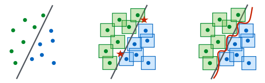
In figure below you can see that when L-infinity perturbations are exercised, there are some examples being misclassified shown in red stars. In higher dimensional data, there is even more possibility to manipulate an input to cross a decision boundary(6).
 (6)
(6) (7)
(7)
figure 3: Non-robust decision boundary (black) and robust one (red) on L-infinity perturbation(6) figure 4: L-p norms on distance 1(7)
You can also see that robust classifier (red line) is more complex than non-robust one (black line). Therefore, capacity of a model is important to be robust, a simple linear regression can construct black line but for red line we need more complex models(6). In addition, robust model is data hungry since without original blue/green dots of corresponding red stars, we wouldn't see adversarial examples(8).
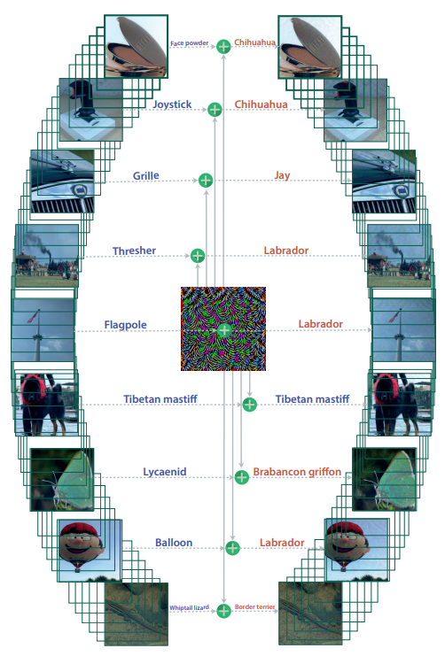
2.2 Universal Adversarial Perturbations (UAPs)
figure 5: UAPs changing multiple labels with one noise(9) |
|
|---|


3. Why models are affected by adversarial examples?
There are several explanations on the root cause of adversarial examples. To my knowledge best explanation in the field is the work of Ilyas, Andrew et. al. This section is focused on their work.
"Adversarial vulnerability is a direct result of our models' sensitivity to well-generalizing features in the data." (1)
Due to our way of constructing supervised learning, models are conditioned to perform best without any constraints. In the standard training setting with the cross-entropy loss or losses alike, loss function doesn't distinguish between robust and non-robust features. This can results in models to pick up any pattern they see in the data if they help model to increase accuracy, without thinking long term(1). In addition, non-robust models have excessive piecewise linearity which means no smooth region on parameter space. Causing outputs to jump another region and misclassify the input(17).
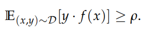
Ilyas et al splıt features into 3 categories: robust-useful, non-robust useful and not useful features. Usefulness in here is measured by the above formula. Basically it is the measure of the correlation between a feature and target without caring about adversarial perturbations. During creation of a model, our general hope is model will utilize useful features to achieve maximum performance/minimum loss. One can also think usefulness is above zero since if a feature is negatively corelated, taking negative of that feature will be corelated with the target(1).
Saying a feature is useful or not is not so easy, for example will we say a feature is e-5 useful, or will it be a not-useful feature? And will there be a feature with 0 usefulness? So since answering these questions are not straightforward and dependent on data, we can select an arbitrary p as a threshold to classify features as robust or not. If you are interested in selection process in here, you can look at to paper from Ilyas et al(1).
3.1 Robust Features
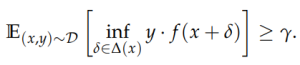
ɣ-robustly p-useful features are defined which are a subset of useful features with resistance to the adversarial perturbations (formula 3.2 below). ɣ here denotes expected resistance to the adversarial perturbations(1).
- Closer to the human perception (looking for tails and ears to identify a cat)
- Stays predictive/useful despite any intervention in the form of perturbation (1)
- Separate clusters which is preserved even under attacks (4)
- More on foreground(3)
Unlike useful features, robust features are actually dependent on the L-p norm we choose. So a feature can be robust in L-1 norm while being non-robust to the L-2 norm. As discussed earlier, you need to select correct L-p norm for your data and accepted tolerance. Like on decision of usefulness, saying a feature is robust or not is not a systematic one. Therefore we can use a threshold to decide whether a feature is robust or not(1). One can decide on this threshold as tolerance level on data. If your predictions being slightly off can cause harm you can increase the threshold but if your meaning of data changes even with slight change on data, maybe you can be good for lower threshold. I think both cases are valid on medical domain.
3.2 Non-Robust Features
p-useful features can also be non-robust. As the name suggests, these features are not ɣ robust and deteriorates under addition of perturbations. Even though these features are helpful to raise the bar for the models, they are not helping in the adversarial robustness(1).
- Features that are mostly incomprehensible to humans (looking for direction and curvature of the fur to identify a cat)
- Brittle(1)
- Generally transferable between models on the same domain(1)
- Takes a large role in standard training settings(1, 3, 4)
- When perturbations on those are small enough, model is still predictive(4)
- Overlapping and disorganized clusters(4)
- More on background(3)
3.3 Detecting Robust & Non-Robust Features
One method is disentangling robust & non-robust features, a disentangled representation layer is used on the input images to create robustified versions. When a model is trained by robustified versions, it is seen that model performs well on both standard test set and adversarial test set with lower accuracy showing use of non-robust features. But this model is more resilient towards attacks than standard one showing brittleness of non-robust features(1).
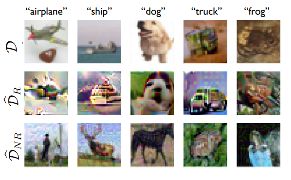
Figure 8: Robustified and non-robustified datasets(1)
Distillation can also be done by Information bottleneck over the intermediate steps of a network. Bottleneck used to regulate the latent feature space by adding noise and measures effects of that noise on different features. Features that are sensitive are attributed as non-robust while others being robust. This again shows brittleness of non-robust features. Information bottleneck here is a reduced representation which is maximally informative representation of the input. This is ensured by additional optimization goal during training(4).
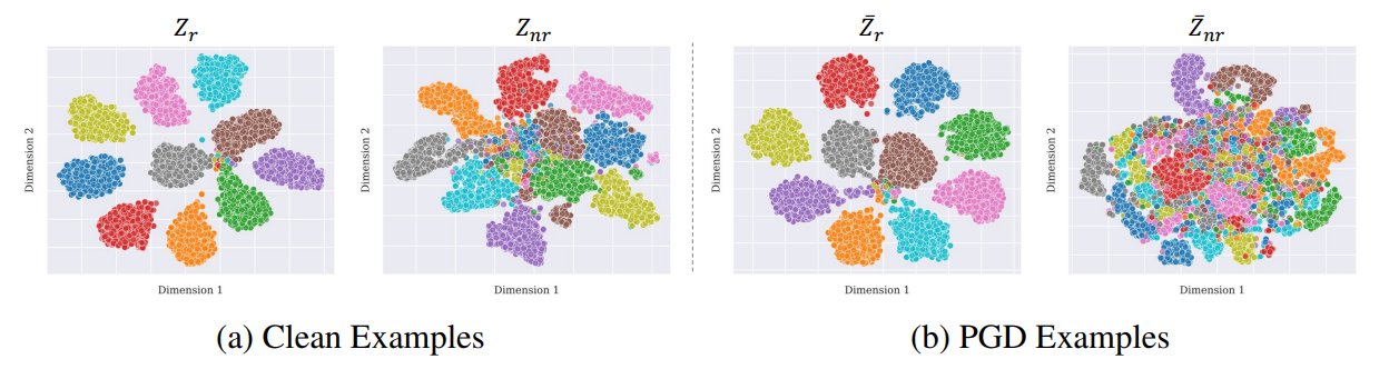
Figure 9: Clustering of features, original ones on left, perturbed ones on right(4)
3.4 Effectiveness of Non-Robust Features
Andrew Ilyas et al. also trained a model with a dataset of adversarial examples. This model still converged even though it lacks robust features but surprisingly it also performs decent on test dataset with correct labels. This shows non-robust features are enough to learn/converge while big models still learning robust features without a label. When the input image lacks non-robust features the model trained on, it used those salient robust features to make the prediction. So that those perturbed images had robust features pointing to the correct class and non-robust features pointing to the false class(1).
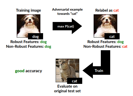
Figure 10: adversarialy trained model(1)
This behavior is not observed at smaller models (like VGG-16) but on bigger models performs (like ResNet-50). Models with higher capacity can learn robust features even though they are not correlated which is confirmed by other studies(1, 2, 3).
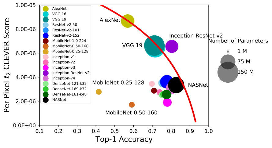
Figure 11: CLEVER score (robustness) vs accuracy (2)
It has been observed adversarialy manipulating non-robust features doesn't visibly change the feature space while you can see some difference on robust features while they preserve their overall structure and outlook(4).
3.4 Can we solve this now? A discussion
So you might be wondering, if we can classify these features and evaluate, can't we prepare for them based on this and solve the issue. Unfortunately, according to some researchers Ilyas et al.'s findings doesn't hold in some cases even though it is reproducible.
Justin Gilmer and Dan Hendrycks connects this behavior to the distributional robustness and points out this effect is still observable on extreme high-pass filtered data. This data is simply a blur of color to the humans without a concrete object. But they argue that this is due to frequency of data and perturbations unlike L-p norm explanation. They have observed models are robust to low-frequency perturbations while it is easier to realize an attack with high-frequency perturbations. And this L-p norm hypothesis introduces a bias and false perception of robustness. Lastly, one other explanation they found to Ilyas's works is distribution shift instead of adversarial robustness(31).
Gabriel Goh argues that model trained on adversarial examples can pick up faint robust features introduced in those adversarial perturbations. Causing robust feature leakage instead of model learning non-useful robust features of the base image. Likewise Eric Wallace shows this can be information leakage from model adversarial examples are generated on to the model that is trained on those adversarial data, not learning salient robust features. Preetum Nakkiran shows generatlization of adversarial examples as not "bugs" is wrong and there is indeed adversarial examples that are just bugs. Bugs in here means they leverage aberrations in the classifier that are not a property of data. It is shown that on the contrary of hypothesis, it is possible to construct adversarial examples even in the case of training data without "non-robust features"(31).
Lastly, Reiichiro Nakano agrees on the findings of Ilyas et al. The same behavior has been observed on style transfer domain too, in particular it is seen that simpler models like VGG works better on style-transfer. Author connected this to the Ilyas's work on robustness and since VGG may not pick up non-robust features, it focuses on robust ones to realize style transfer which turns out more realistic to the humans(31).
In my opinion, one other weak point can be deciding on L-p norms and a specific one for different cases. L-p norms are a good way to formulize perturbations but it creates a norm ball which is more like a circle to a square. However, I believe it is also possible that these perturbations can be valid in a elipsoid rather than a circle. Meaning that data/model may be susceptible in 1 distance on some axes while 2 distance on others. Choosing distance as 1 or 2 in these cases both has some disadvantages like 2 distance can also contain justifiably false predictions like perturbations that change image in a meaningful way to a new class. I believe there is still more to research these features and their behavior under attack schemes.
3.5 Contribution by Regions
According to Xin Wang et al., understanding effects of perturbation goes through understanding partial effects of each region on the image. Their hypothesis is different regions increase or decrease a possibility of attack over the input. To understand this, they have decomposed both perturbation map and the input image into chunks and evaluated effects of each part. Upon that, authors observed strong inter-community connections and cooperation over pixels. This interactions are measured by Shapley values and found that this is mostly correct and a single pixel is not responsible for success of an attack(3).
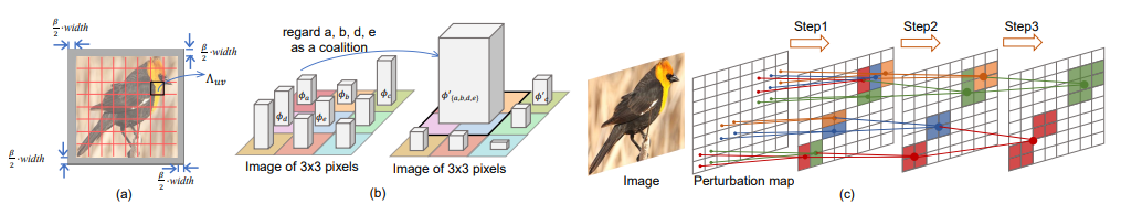
Figure 12: Region pooling by robustness(3)
- Robustness → active on foreground(3)
- Effect of pixels & regions are dependent on the context and neighborhood pixels(3)
- Some patterns are effective towards forming an attack → cooperation(3)
- Shapley values are used(3)
- Approaches like GradCAM are not suitable since they create heat maps based on human perception, which they have seen may not tell the whole story in this setting
- Importance of regions are similar for L-2 and L-inf attacks but overall perturbations observed are significantly different(3)

Figure 13: Effective regions of perturbations(3)
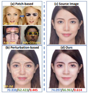
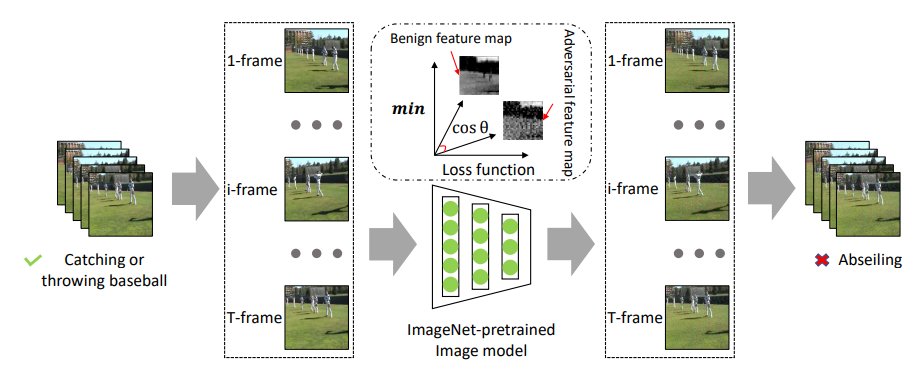
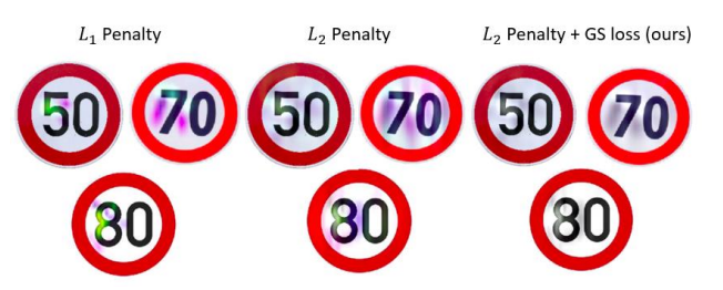
4. Real World Examples
Figure 14: Adversarial make-up to fool face detectors(12) |
Figure 15: Video models effected by perturbing frames(13) |
Figure 16: Adversarial cloths make people invisible(14) |
Figure 17: Speed signs can be painted to fool models(15)
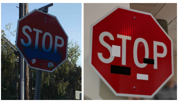
Figure 18: Putting stickers on STOP signs make them speed signs for models(16) |

Also, perturbations found at parent model and/or a similar model (domain or structure wise) can effect your model.
5. Some of the prominent defenses
You can find a list of defenses proposed at CVPR21 & CVPR22 with my own categorization below. Most of the mentioned approaches are not silver bullet to the robustness problem and many of them are considered in only one L-p setting as robust.
| Out of model defenses | On model defenses (strengthen model) | On model defenses (rejection) |
|---|---|---|
| Towards Practical Certifiable Patch Defense With Vision Transformer(20) | Enhancing Adversarial Robustness for Deep Metric Learning(18) | Two Coupled Rejection Metrics Can Tell Adversarial Examples Apart(19) |
| LiBRe(22) | ShapPruning(21) | |
| CLEVER(29) | Architectural Adversarial Robustness: The Case for Deep Pursuit(23) | |
Adversarial Training(25,26) |
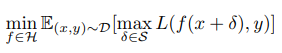
Adversarial Training
This can be thought as a min-max game from the game theory. Adversary tries to maximize loss while defender tries to minimize that maximal loss. Basic idea is to show perturbed images to the classifier so that it can get ready for them and learn a classifier in a robust manner. This can also be thought as a data augmentation(25,26).
 (25)
(25)
 (24)
(24)
7. References
(1) Ilyas, Andrew, et al. "Adversarial examples are not bugs, they are features." Advances in neural information processing systems 32 (2019).
(2) Su, Dong, et al. "Is Robustness the Cost of Accuracy?--A Comprehensive Study on the Robustness of 18 Deep Image Classification Models." Proceedings of the European Conference on Computer Vision (ECCV). 2018.
(3) Wang, Xin, et al. "Interpreting attributions and interactions of adversarial attacks." Proceedings of the IEEE/CVF International Conference on Computer Vision. 2021.
(4) Kim, Junho, Byung-Kwan Lee, and Yong Man Ro. "Distilling robust and non-robust features in adversarial examples by information bottleneck." Advances in Neural Information Processing Systems 34 (2021): 17148-17159.
(5) Gong, Yuan, and Christian Poellabauer. "Protecting voice controlled systems using sound source identification based on acoustic cues." 2018 27th International Conference on Computer Communication and Networks (ICCCN). IEEE, 2018.
(6) Madry, Aleksander, et al. "Towards deep learning models resistant to adversarial attacks." arXiv preprint arXiv:1706.06083 (2017).
(7) "Unit circles of different p -norms in two dimensions." Figure. Wikimedia, Wikimedia Commons, 17 Oct. 2018, de.wikipedia.org/wiki/P-Norm#/media/Datei:Vector-p-Norms_qtl1.svg.
(8) Schmidt, Ludwig, et al. "Adversarially robust generalization requires more data." Advances in neural information processing systems 31 (2018).
(9) Moosavi-Dezfooli, Seyed-Mohsen, et al. "Universal adversarial perturbations." Proceedings of the IEEE conference on computer vision and pattern recognition. 2017.
(10) Park, Sung Min, et al. "On Distinctive Properties of Universal Perturbations." arXiv preprint arXiv:2112.15329 (2021).
(11) Salman, Hadi, et al. "Unadversarial examples: Designing objects for robust vision." Advances in Neural Information Processing Systems 34 (2021): 15270-15284.
(12)Hu, Shengshan, et al. "Protecting Facial Privacy: Generating Adversarial Identity Masks via Style-robust Makeup Transfer." Proceedings of the IEEE/CVF Conference on Computer Vision and Pattern Recognition. 2022.
(13)Wei, Zhipeng, et al. "Cross-Modal Transferable Adversarial Attacks from Images to Videos." Proceedings of the IEEE/CVF Conference on Computer Vision and Pattern Recognition. 2022.
(14)Hu, Zhanhao, et al. "Adversarial Texture for Fooling Person Detectors in the Physical World." Proceedings of the IEEE/CVF Conference on Computer Vision and Pattern Recognition. 2022.
(15)Morgulis, Nir, et al. "Fooling a real car with adversarial traffic signs." arXiv preprint arXiv:1907.00374 (2019).
(16)Eykholt, Kevin, et al. "Robust physical-world attacks on deep learning visual classification." Proceedings of the IEEE conference on computer vision and pattern recognition. 2018.
(17)Engstrom, Logan, et al. "Exploring the landscape of spatial robustness." International conference on machine learning. PMLR, 2019.
(18)Zhou, Mo, and Vishal M. Patel. "Enhancing Adversarial Robustness for Deep Metric Learning." Proceedings of the IEEE/CVF Conference on Computer Vision and Pattern Recognition. 2022.
(19)Pang, Tianyu, et al. "Two Coupled Rejection Metrics Can Tell Adversarial Examples Apart." Proceedings of the IEEE/CVF Conference on Computer Vision and Pattern Recognition. 2022.
(20)Chen, Zhaoyu, et al. "Towards Practical Certifiable Patch Defense with Vision Transformer." Proceedings of the IEEE/CVF Conference on Computer Vision and Pattern Recognition. 2022.
(21)Guan, Jiyang, et al. "Few-shot Backdoor Defense Using Shapley Estimation." Proceedings of the IEEE/CVF Conference on Computer Vision and Pattern Recognition. 2022.
(22)Deng, Zhijie, et al. "Libre: A practical bayesian approach to adversarial detection." Proceedings of the IEEE/CVF Conference on Computer Vision and Pattern Recognition. 2021.
(23)Cazenavette, George, Calvin Murdock, and Simon Lucey. "Architectural adversarial robustness: The case for deep pursuit." Proceedings of the IEEE/CVF Conference on Computer Vision and Pattern Recognition. 2021.
(24)Zheng, Haizhong, et al. "Efficient adversarial training with transferable adversarial examples." Proceedings of the IEEE/CVF Conference on Computer Vision and Pattern Recognition. 2020.
(25)Aleksander Madry, Aleksandar Makelov, Ludwig Schmidt, Dimitris Tsipras, and Adrian Vladu. Towards deep learning models resistant to adversarial attacks. In International Conference on Learning Representations (ICLR), 2018.
(26)Madry, Alexander, and Zico Kolter. "J. Z. Kolter and A. Madry: Adversarial Robustness - Theory and Practice." NeurIPS 2018 Tutorial, 7 Dec. 2018, Speech.
(27)Yamada, Yutaro, and Mayu Otani. "Does Robustness on ImageNet Transfer to Downstream Tasks?." Proceedings of the IEEE/CVF Conference on Computer Vision and Pattern Recognition. 2022.
(28)Salman, Hadi, et al. "Do adversarially robust imagenet models transfer better?." Advances in Neural Information Processing Systems 33 (2020): 3533-3545.
(29)Weng, Tsui-Wei, et al. "Evaluating the robustness of neural networks: An extreme value theory approach." arXiv preprint arXiv:1801.10578 (2018).
(30)Engstrom, Logan, et al. "Exploring the landscape of spatial robustness." International conference on machine learning. PMLR, 2019.
(31)Engstrom, et al., "A Discussion of 'Adversarial Examples Are Not Bugs, They Are Features'", Distill, 2019.