Blog post written by: Mahir Efe Kaya
Based on:Dor Bank, Noam Koenigstein, Raja Giryes, "Autoencoders," in arXiv:2003.05991
Autoencoders are a fascinating branch of neural networks designed to learn efficient codings of input data. This post delves into the various aspects of autoencoders, focusing on their types, functionalities, and applications, explained in an accessible manner.
1. What Are Autoencoders?
Autoencoders are neural networks that aim to learn a representation (encoding) for a set of data, typically for the purpose of dimensionality reduction or feature learning. The network is trained to map input data to itself through a process that involves two main components:
- Encoder: Compresses the input into a latent-space representation.
- Decoder: Reconstructs the input from the compressed representation.
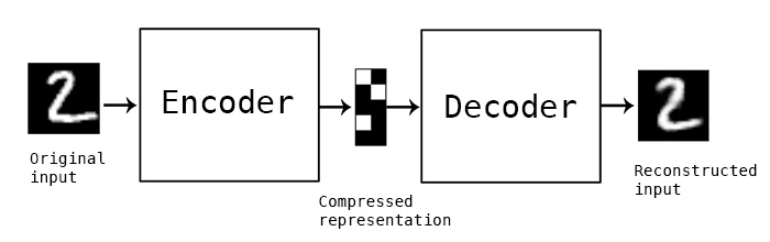
The primary objective is to minimize the difference between the original input and the reconstructed output, which is measured by a loss function, often the mean squared error (MSE).
Mathematically, this can be represented as:
| argmin_A_,_BE[Δ(x,B∘A(x))] |
where:
- A is the encoding function (encoder).
- B is the decoding function (decoder).
- x is the input data.
- B∘A(x) is the reconstructed data.
- Δ(x,B∘A(x)) is the reconstruction loss function, such as mean squared error.
- E denotes the expected value over the distribution of input data.
Autoencoders can be visualized as a bottleneck structure where the input data is squeezed into a compact form before being expanded back to its original size. This bottleneck forces the network to learn the most critical features of the data.
2. Regularized Autoencoders:
These techniques prevent overfitting and ensure meaningful representations, thus avoiding trivial solutions such as the identity function.Common methods include:
2.1. Sparse Autoencoders:
Sparse autoencoders extend the basic autoencoder architecture by adding a sparsity constraint to the hidden layer. This constraint forces the model to use only a small number of active neurons to represent the input, promoting the learning of meaningful features.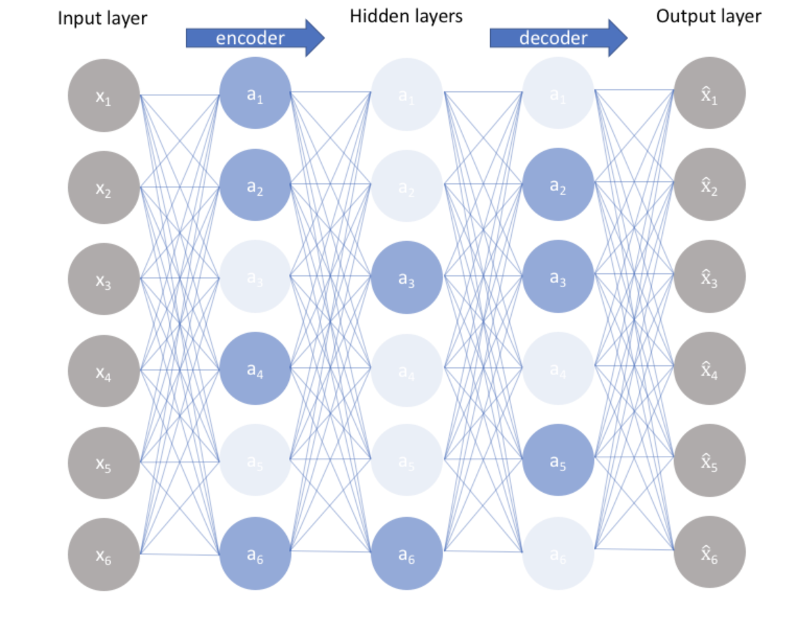
The process can be broken down into three main steps:
- Encoding: Compress the input into a latent-space representation with a constraint on sparsity.
- Decoding: Reconstruct the input from the sparse latent representation.
- Sparsity Constraint: Apply a penalty to ensure that the activation of neurons in the hidden layer remains sparse, like a percentage of activated neurons in one layer.
By learning to use only a few active neurons, sparse autoencoders can capture essential features of the data, leading to more interpretable and useful representations. To enforce sparsity, the loss function evolves into this:
| \arg \min_{A, B} \mathbb{E}[\Delta(x, B \circ A(x))] + \sum_j \text{KL}(p \| \hat{\rho}_j) |
where:
- the first term is construction loss
- the second term, \text{KL}(p \| \hat{\rho}_j), represents the sparsity constraint and ensures that the average activation of each hidden unit jj is close to the sparsity target pp. The Kullback-Leibler (KL) divergence measures how much the actual average activation \hat{p_j} deviates from the target sparsity:
- is the desired sparsity level, typically a small value indicating that the hidden units should be active only a small fraction of the time.
- \hat{p_j} is the average activation of the hidden unit j over the training data.
2.2. Denoising Autoencoders:
Denoising autoencoders are an extension of the basic autoencoder architecture. While traditional autoencoders learn to reconstruct the input data from a compressed representation, denoising autoencoders are trained to reconstruct the original, noise-free data from a corrupted version of the input. This additional challenge encourages the model to capture more robust features that are less sensitive to noise.

The process can be broken down into three main steps:
- Corruption: Introduce noise to the input data, creating a corrupted version of the input.
- Encoding: Compress the corrupted input into a latent-space representation.
- Decoding: Reconstruct the original, noise-free input from the latent representation.
By learning to remove noise from the data, denoising autoencoders improve the model's ability to generalize to new, unseen data.
2.3. Contractive Autoencoders:
Contractive Autoencoders (CAEs) enhance traditional autoencoders by adding a penalty to the loss function, making the encoding less sensitive to small changes in the input. This promotes robust and stable representations that capture essential data structures. This is done by penalizing the Jacobian matrix of the encoder's output with respect to its input, encouraging the model to learn a stable representation.
Key Features
Robustness to Perturbations: CAEs produce representations that are robust to small input changes by penalizing the sensitivity of the encoder’s output.
Stability in Latent Space: CAEs ensure that similar inputs map to nearby points in the latent space, maintaining consistency and meaningful representations.
Mathematical Formulation
The loss function for CAEs includes a reconstruction loss and a contractive penalty:
| \[ \arg \min_{A, B} \mathbb{E}[\Delta(x, B \circ A(x))] + \lambda \|J_f(x)\|_F^2 \] |
- \Delta(x, B \circ A(x)) is the reconstruction loss function, such as mean squared error.
- \|J_f(x)\|_F is the Frobenius norm of the Jacobian matrix of the encoder.
- \lambda is a regularization parameter controlling the importance of the contraction penalty.
Contractive Autoencoders provide a robust and stable alternative to traditional autoencoders. By penalizing the sensitivity of the encoder's output, CAEs ensure that the learned representations are reliable and less affected by noise, making them useful for a wide range of applications involving noisy or perturbed data.
3. Variational Autoencoders (VAEs):
Variational Autoencoders (VAEs) represent a significant advancement in the field of generative models. Unlike traditional autoencoders that learn a deterministic mapping from input to a latent space, VAEs learn a probabilistic mapping. This section delves deeper into the mechanics, mathematics, and significance of VAEs.
3.1. The Generative Process
The fundamental idea behind VAEs is to model the data generation process. We assume that data is generated by a process involving a set of latent variables. The goal is to learn the distribution of these latent variables and use them to generate new data.
Formally, given an observed dataset \mathbf{X} = \{\mathbf{x}_i\}_{i=1}^N, consisting of N samples, we assume that each data point \mathbf{x}_i is generated from a latent variable \mathbf{z}_i according to a prior distribution and a likelihood function p_θ(x∣z), parameterized by θ.
3.2. Variational Inference
The key challenge in VAEs is to compute the posterior distribution p_θ(z∣x). Direct computation is intractable due to the complex integral over the latent space. Variational inference provides a solution by introducing an approximate posterior distribution q_ϕ(z∣x), parameterized by ϕ.
The objective is to make the approximate posterior q_ϕ(z∣x) close to the true posterior p_θ(z∣x). This is achieved by maximizing the Evidence Lower Bound (ELBO):
| \(\log p_\theta(\mathbf{x}) \geq \mathbb{E}_{q_\phi(\mathbf{z}|\mathbf{x})} \left[ \log p_\theta(\mathbf{x}|\mathbf{z}) \right] - D_{\text{KL}} \left( q_\phi(\mathbf{z}|\mathbf{x}) \| p(\mathbf{z}) \right)\) |
Here,D_{KL} denotes the Kullback-Leibler divergence, which measures the difference between the approximate posterior and the prior distribution. The ELBO can be expanded as:
| \(\mathcal{L}(\theta, \phi; \mathbf{x}) = \mathbb{E}_{q_\phi(\mathbf{z}|\mathbf{x})} \left[ \log p_\theta(\mathbf{x}|\mathbf{z}) \right] - D_{\text{KL}} \left( q_\phi(\mathbf{z}|\mathbf{x}) \| p(\mathbf{z}) \right)\) |
Maximizing the ELBO involves two terms:
- Reconstruction Term: Encourages the model to reconstruct the input data accurately from the latent representation.
- KL Divergence Term: Regularizes the latent space to match the prior distribution.
3.3. Reparameterization Trick
To optimize the ELBO using gradient-based methods, we need to backpropagate through the stochastic sampling of z. The reparameterization trick simplifies this by expressing the sampling process as a deterministic function of the input and some auxiliary noise variable ϵ:
| \(\mathbf{z} = \mu_\phi(\mathbf{x}) + \sigma_\phi(\mathbf{x}) \odot \mathbf{\epsilon}\) |
Here, μ_ϕ and σ_ϕ are the outputs of the encoder network representing the mean and standard deviation of the approximate posterior, and ϵ is a standard normal noise.
This transformation allows gradients to flow through the sampling process, enabling efficient optimization of the VAE.
3.4. The Complete VAE Model
The VAE consists of two neural networks:
- Encoder (Recognition Network): Approximates the posterior q_ϕ(z∣x). It outputs the mean and standard deviation σ_ϕ of the latent distribution.
- Decoder (Generative Network): Models the likelihood . It takes a sample from the latent distribution and generates a reconstruction of the input.

The overall training objective is to maximize the ELBO for each data point in the training set.
3.5. Mathematical Formulation
The encoder network outputs μ_ϕ(x) and , defining a Gaussian distribution \(q_\phi(\mathbf{z}|\mathbf{x}) = \mathcal{N}(\mathbf{z}; \mu_\phi(\mathbf{x}), \sigma_\phi(\mathbf{x}))\). The decoder network defines the likelihood , which is often modeled as a Gaussian distribution with mean and fixed variance:
| \(p_\theta(\mathbf{x}|\mathbf{z}) = \mathcal{N}(\mathbf{x}; \nu_\theta(\mathbf{z}), \mathbf{I})\) |
The loss function to be minimized is the negative ELBO:
| \(\mathcal{L}(\theta, \phi; \mathbf{x}) = - \mathbb{E}_{q_\phi(\mathbf{z}|\mathbf{x})} \left[ \log p_\theta(\mathbf{x}|\mathbf{z}) \right] + D_{\text{KL}} \left( q_\phi(\mathbf{z}|\mathbf{x}) \| p(\mathbf{z}) \right)\) |
This loss function balances the reconstruction quality and the regularization of the latent space.
4. Disentangled Autoencoders:
Disentangled autoencoders build on variational autoencoders by introducing a parameter ββ that scales the KL divergence term. This modification promotes the separation of factors of variation in the latent space, ensuring each latent dimension captures a distinct and meaningful aspect of the data.
| \[ \mathcal{L}(\theta, \phi, \mathbf{x}^{(i)}) = \mathbb{E}_{q_\phi(z|\mathbf{x}^{(i)})}[\log p_\theta(\mathbf{x}^{(i)}|z)] - \beta D_{KL}(q_\phi(z|\mathbf{x}^{(i)}) \| p_\theta(z)). \] |
- β is a regularization parameter controlling the importance of the KL divergence term.
In this setup, the KL divergence term regularizes the latent feature distribution q_ϕ(z∣x) to be less correlated, promoting disentanglement. Increasing β results in more disentangled (less correlated) features.
5. Applications of Autoencoders
Autoencoders have a wide range of applications across various domains:
5.1. Generative Models
Variational autoencoders (VAEs) generate new data samples by learning a probabilistic distribution over the data, which allows them to create new instances that resemble the training data. This capability is particularly useful in applications such as image and text generation, where the goal is to produce new, realistic samples based on the learned distribution. VAEs achieve this by encoding the input data into a latent space characterized by a mean and variance, from which new samples can be drawn. The latent space is structured so that similar points correspond to similar data outputs, enabling smooth interpolation and meaningful variations between data points.

This process involves a probabilistic framework that allows for the generation of diverse and novel samples, making VAEs valuable for tasks that require synthetic data generation, such as creating new product designs, generating artistic content, and augmenting datasets to train more robust machine learning models. The ability to generate realistic data opens up numerous possibilities for creative and practical applications, providing a powerful tool for data synthesis and enhancement.
5.2. Classification
Autoencoders can significantly improve classification performance, especially in semi-supervised learning settings where labeled data is scarce but unlabeled data is abundant. By learning compact and informative representations of the input data, autoencoders help in extracting essential features that enhance the accuracy of classifiers. The encoder component of an autoencoder compresses the high-dimensional input data into a lower-dimensional latent space that retains critical information. This compressed representation can then be used as input to a classifier, which benefits from the reduced dimensionality and the highlighted relevant features.
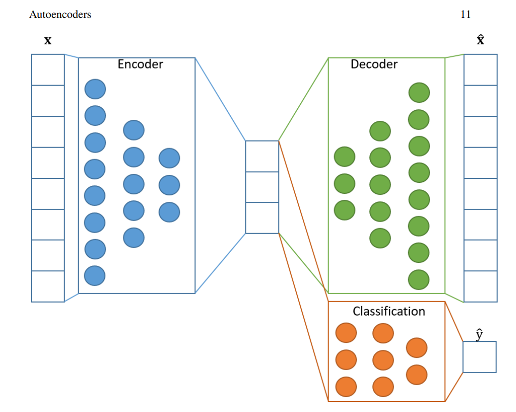
The process not only simplifies the data but also improves the classifier's ability to distinguish between different classes, leading to better overall performance. This approach is particularly beneficial in scenarios where obtaining labeled data is challenging, allowing the model to leverage the abundant unlabeled data to improve classification accuracy. By providing a richer feature set, autoencoders contribute to more robust and effective classification models.
5.3. Clustering
Autoencoders facilitate clustering by learning compact data representations that capture the underlying structure of the data. By transforming high-dimensional data into a lower-dimensional latent space, autoencoders make it easier to apply clustering algorithms effectively. The latent space representation ensures that similar data points are closer together, enhancing the accuracy of clustering algorithms like k-means or hierarchical clustering.
This method is particularly useful for handling high-dimensional datasets, where traditional clustering methods struggle. Improved clustering performance benefits various applications, such as customer segmentation, image classification, and gene expression analysis, by revealing natural groupings within the data. The process involves training the autoencoder to capture the essential features of the data in its latent space, which can then be fed into standard clustering algorithms to identify meaningful clusters. This approach not only simplifies the clustering task but also improves the reliability and interpretability of the results, making it a powerful tool for data analysis and segmentation.
5.4. Anomaly Detection
Autoencoders can effectively identify anomalies by learning the typical representation of normal data and detecting deviations from this norm. When the model is trained on normal data, it minimizes the reconstruction error for these patterns. However, when it encounters abnormal or unseen data, the reconstruction error increases significantly, flagging it as an anomaly. This approach is useful in applications like fraud detection, where unusual patterns can indicate fraudulent activity, and industrial monitoring, where detecting equipment malfunctions early can prevent costly downtimes. By focusing on deviations from the learned normal patterns, autoencoders provide a robust method for anomaly detection across various fields. The high reconstruction error for anomalous data points makes it easy to identify outliers, ensuring timely intervention and improving operational safety and reliability. This method offers an efficient and automated way to monitor systems and detect irregularities, making it a valuable tool for maintaining the integrity and security of various applications.
5.5. Recommendation Systems
A recommender system predicts users' preferences for items and is widely used in e-commerce, app stores, and online content platforms. Collaborative Filtering (CF) is a common approach, inferring user preferences based on the preferences of similar users, assuming people with similar past preferences will have similar future preferences.
Autoencoders are utilized in recommender systems through the AutoRec model, which has two variants: user-based AutoRec (U-AutoRec) and item-based AutoRec (I-AutoRec). U-AutoRec learns a compact representation of item preferences for specific users, while I-AutoRec learns user preferences for specific items.
For example, with M users and N items, let r_m∈R^N be the preference vector for user m. In U-AutoRec, the decoder z=g(r_m) maps r_m to a lower-dimensional vector z∈R^d, where d≪N. The encoder reconstructs the preferences as h(r_m; \theta) = f(g(r_m)), with θ as the model’s parameters. The U-AutoRec objective is:
| \arg \min_{\theta} \sum_{m=1}^M \| r_m - h(r_m; \theta) \|_O^2 + \lambda \cdot \text{reg} |
In I-AutoRec, let m be the preference vector for item n. The I-AutoRec objective is:
| \arg \min_{\theta} \sum_{n=1}^N \| r_n - h(r_n; \theta) \|_O^2 + \lambda \cdot \text{reg} |
5.6. Dimensionality Reduction
Autoencoders reduce the dimensionality of data while preserving important information, similar to Principal Component Analysis (PCA) but with the added capability to capture non-linear relationships. This is achieved through the encoder, which compresses the input data into a lower-dimensional latent space, and the decoder, which reconstructs the original data from this compact representation. Dimensionality reduction is particularly useful in visualizing high-dimensional data, enabling better understanding of underlying patterns and structures. By retaining essential information in a more manageable form, autoencoders facilitate efficient data analysis and preprocessing for other machine learning models. This approach is beneficial in applications such as feature extraction, noise reduction, and visualization, where reducing the number of dimensions helps in interpreting the data more effectively. The ability to transform complex, high-dimensional data into a simpler form while maintaining its integrity makes autoencoders a valuable tool for exploratory data analysis and model training. This process enhances the usability of data by simplifying it and highlighting the most critical features, enabling more accurate and insightful analysis.
6. Advanced Techniques
Autoencoders, fundamental models in unsupervised learning, have been significantly enhanced through the integration of various advanced techniques. These enhancements address the limitations of traditional autoencoders, improve their performance, and expand their applicability. Below, we explore in detail several sophisticated techniques that have greatly enhanced the capabilities of autoencoders.
6.1. Generative Adversarial Networks (GANs)
Combining autoencoders with Generative Adversarial Networks (GANs) has led to substantial improvements in the quality of generated data. A GAN architecture typically consists of two parts: a generator, which creates new samples, and a discriminator, which distinguishes between real and generated samples. This adversarial training involves the generator aiming to produce data indistinguishable from real samples, while the discriminator learns to accurately differentiate between real and fake data. The benefits include:
- Sharper Outputs: The adversarial loss encourages the generator to produce more detailed and realistic outputs, reducing blurriness.
- Improved Realism: The discriminator's feedback helps the generator create data closer to real samples, suitable for high-quality applications like image and video synthesis.
Different approaches have been developed to combine the strengths of autoencoders and GANs. For example, Adversarial Autoencoders (AAE) replace the KL-divergence in the VAE loss function with a discriminator network. This discriminator distinguishes between the prior and the approximated posterior, leading to more realistic generated samples. Another approach merges the reconstruction loss in VAE with a discriminator, making the decoder essentially function as the generator. Combining the discriminator of GANs with an encoder via shared weights enables the latent space to be conveniently modeled for inference, enhancing the realism of generated outputs.
6.2. Adversarially Learned Inference (ALI)
Adversarially Learned Inference (ALI) attempts to merge the strengths of VAEs and GANs, achieving a balance between their strengths and weaknesses. Instead of using a traditional loss function, ALI employs a discriminator to distinguish between pairs (x,\hat{z}), where x is an input sample and \hat{z} \sim q(z \mid x) is sampled from the encoder’s output, and (\tilde{x}, z) pairs, wherez∼p(z) is sampled from the prior and \tilde{x} \sim p(x \mid z) is the decoder's output. This approach forces the decoder to produce realistic outputs to "fool" the discriminator while maintaining the autoencoder structure. ALI allows for meaningful alterations in images by enabling specific feature manipulation in the latent space.
6.3. Wasserstein Autoencoders (WAEs)
Wasserstein Autoencoders (WAEs) use the Wasserstein distance as a loss function, offering better convergence properties and more stable training. The Wasserstein distance measures the cost of transforming one probability distribution into another, providing a meaningful measure of discrepancy between distributions. This approach has several advantages:
- Stable Training: The Wasserstein distance provides a smoother gradient, leading to more stable and faster convergence during training.
- Meaningful Latent Space: WAEs ensure that the latent space is structured so that similar points correspond to similar data, facilitating tasks like interpolation and data synthesis.

The WAE objective function includes a reconstruction loss that penalizes the output distribution relative to the sample distribution and a regularization term that penalizes the distance between the latent space distribution and the prior distribution. This method promotes better utilization of the latent space and improves the quality of generated samples.
The mathematical formulation for the Wasserstein distance used in WAEs is:
| W_c(P_X, P_G) = \inf_{\Gamma \in \Pi(P_X, P_G)} \mathbb{E}_{(X, Y) \sim \Gamma} [c(X, Y)] |
where c(x,y) is a cost function, and Γ is the set of all joint distributions whose marginals are P_X and P_G. Whenc(x,y)=d(x,y), the 1-Wasserstein distance (also known as the "Earth Moving Distance") is defined as:
| W_1(P_X, P_G) = \sup_{f \in \mathcal{F}} \mathbb{E}_{X \sim P_X} [f(X)] - \mathbb{E}_{Y \sim P_G} [f(Y)] |
6.4. Deep Feature Consistent Variational Autoencoder (DFC-VAE)
Deep Feature Consistent Variational Autoencoders (DFC-VAE) enhance traditional autoencoder frameworks by incorporating perceptual quality into the reconstruction process. Unlike conventional methods that focus solely on minimizing pixel-wise differences, DFC-VAE leverages features from pre-trained networks to ensure that reconstructions are close in both pixel space and feature space.
This approach emphasizes two main aspects:
- Perceptual Quality: By using features from pre-trained networks, DFC-VAE ensures that reconstructed images align with high-level features perceived by humans. This results in outputs that are more visually appealing and realistic.
- Feature Space Alignment: Using deep features helps preserve important structural and semantic details of the original data. This method maintains the integrity of complex patterns and relationships within the data, leading to higher quality reconstructions.
The process involves using a pre-trained classification network as a feature extractor to measure differences between the original and reconstructed images at various layers. This ensures that the reconstructions are more realistic and retain crucial details.
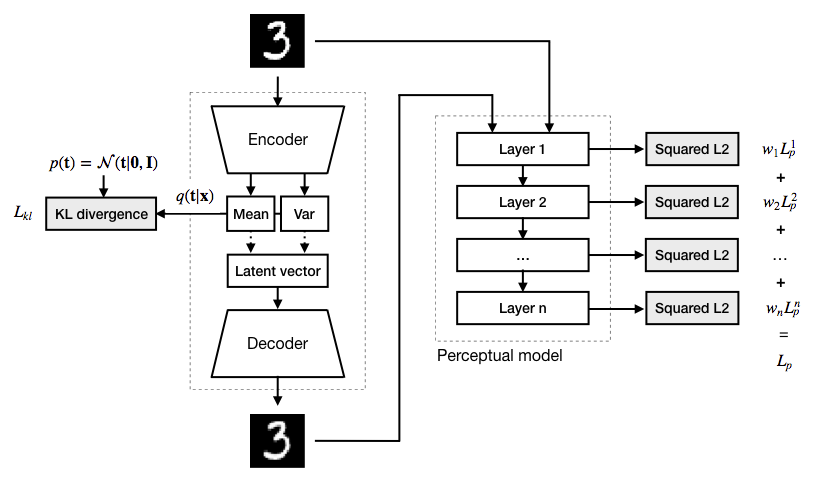
The provided diagram illustrates the architecture of DFC-VAE. The input image is encoded into a latent vector by the encoder, which outputs the mean and variance. This latent vector is sampled and passed to the decoder, which reconstructs the image. Both the original and reconstructed images are fed through a pre-trained perceptual model, extracting features from various layers. The perceptual loss is computed based on the differences in these features, ensuring that the reconstructed image aligns closely with the original in both pixel and feature space. This combination of pixel-wise and perceptual losses results in reconstructions that are not only accurate in terms of pixel values but also maintain high-level structural and semantic details.
6.5. PixelCNN Decoders
Incorporating PixelCNN into the decoder architecture leverages the local spatial statistics of images. PixelCNN models the dependencies between pixels by generating images sequentially and considering the context provided by previously generated pixels. This method reduces blur and improves coherence, offering several benefits:
- Reduced Blur: PixelCNN decoders significantly reduce blur by capturing local pixel dependencies, resulting in sharper images.
- Coherent Outputs: The ability to model pixel dependencies ensures that generated images are coherent and realistic.

PixelCNN works by ordering the pixels in an image in a specific sequence (e.g., top to bottom, left to right). Each pixel is predicted based on the previous pixels and the input image, taking into account local spatial dependencies. For example, in PixelCNN, the probability of a pixel being a certain color is influenced by the colors of neighboring pixels. This sequential generation process helps in maintaining the local structure and coherence of the images.
7. Conclusion
Autoencoders are a versatile tool in the field of machine learning, with applications ranging from data compression to anomaly detection and generative modeling. The continuous evolution of their architectures and techniques promises even greater capabilities and applications in the future. By understanding and leveraging these powerful networks, we can address complex challenges in data processing and representation.
As research progresses, we can expect further improvements in the robustness, efficiency, and interpretability of autoencoders, making them even more integral to various machine learning and data science tasks. For instance, advancements in combining autoencoders with other models, such as GANs and VAEs, have already shown significant potential in generating high-quality data, enhancing feature extraction, and improving anomaly detection. These hybrid models are likely to become more refined, providing even more precise and reliable results.
The integration of autoencoders with sophisticated loss functions, such as those utilizing perceptual models and the Wasserstein distance, has also paved the way for more realistic and detailed reconstructions. This is particularly important in fields like medical imaging, where the accuracy of reconstructions can have a direct impact on diagnostic outcomes.
Moreover, the ability of autoencoders to learn compact and informative representations of data makes them invaluable for dimensionality reduction and clustering, facilitating better visualization and understanding of high-dimensional data. This capability is crucial for exploratory data analysis and can significantly enhance the performance of subsequent machine learning models.
In the realm of generative modeling, autoencoders, especially VAEs, have shown remarkable success in creating new data samples that closely resemble the training data. This opens up exciting possibilities for creative applications, such as art and music generation, as well as practical uses in data augmentation and synthetic data generation for training robust machine learning models.
Autoencoders' role in recommendation systems is also noteworthy, as they enable the creation of personalized recommendations by learning latent representations of user-item interactions. This leads to more accurate and relevant suggestions, enhancing user experience in various online platforms.
Whether you're a researcher exploring the theoretical underpinnings of autoencoders or a practitioner applying these models to solve real-world problems, the field of autoencoders offers a rich and exciting landscape of opportunities. Continued innovation and interdisciplinary collaboration will likely drive further advancements, solidifying autoencoders as a cornerstone of modern AI and machine learning.
In conclusion, autoencoders are more than just a neural network architecture; they represent a powerful framework for understanding and manipulating complex data. Their ability to transform data into meaningful representations and generate high-quality outputs makes them a critical component of the AI toolbox. As we continue to explore their potential and develop new techniques, autoencoders will undoubtedly play a pivotal role in shaping the future of artificial intelligence and data science.