Adapting classifiers for dense prediction
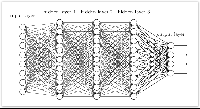
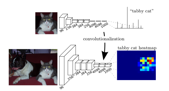
Typical recognition nets, including LeNet , AlexNet [5], ostensibly take fixed-sized inputs and produce non-spatial outputs. The fully connected layers of these nets have fixed dimensions and throw away spatial coordinates. However, these fully connected layers can also be viewed as convolutions with kernels that cover their entire input regions. Doing so casts them into fully convolutional networks that take input of any size and output classification maps. This transformation is illustrated in the figure on the right (figure 6).
For example, for the normal convolutional network deal with classification tasks, there will be some fully connected layers at the end of network, the output of fully connected layers pass through the soft-max function, several probabilities are generated, the input image will be classified into the class which has highest probability. For a fully convolutional network, fully connected layers are replaced by convolutional layers, the spatial output maps of these convolutionalized models make them a natural choice for dense problems like semantic segmentation.
Upsampling is backwards strided convolution
A way to connect coarse outputs to dense pixels is interpolation. For instance, simple bilinear interpolation computes each output from the nearest four inputs by a linear map that depends only on the relative positions of the input and output cells. In a sense, upsampling with factor f is convolution with a fractional input stride of 1/f . So long as f is integral, a natural way to upsample is therefore backwards convolution (sometimes called deconvolution) with an output stride of f. Note that the deconvolution filter in such a layer need not be fixed, but can be learned.
Segmentation Architecture based on VGG
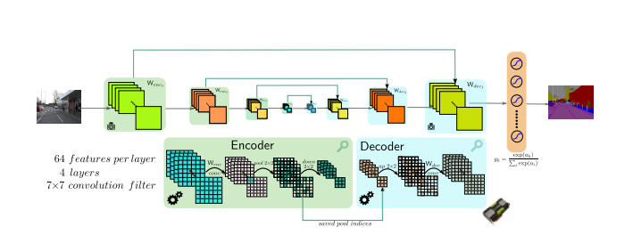
VGG neural network did exceptionally well in ImageNet Large Scale Visual Recognition Competition 2014. The fully connected layers of VGG are replaced by convolutional layers, after the input image pass through the original 5 convolutional layers of VGG, it will be upsampled by 2 deconvolutional layers to generate a output image with the same size as input image. For each pixel, it will be inputted to the soft-max function, every pixel will be classified into the class with highest probability, and illustrated with different color in the output image.
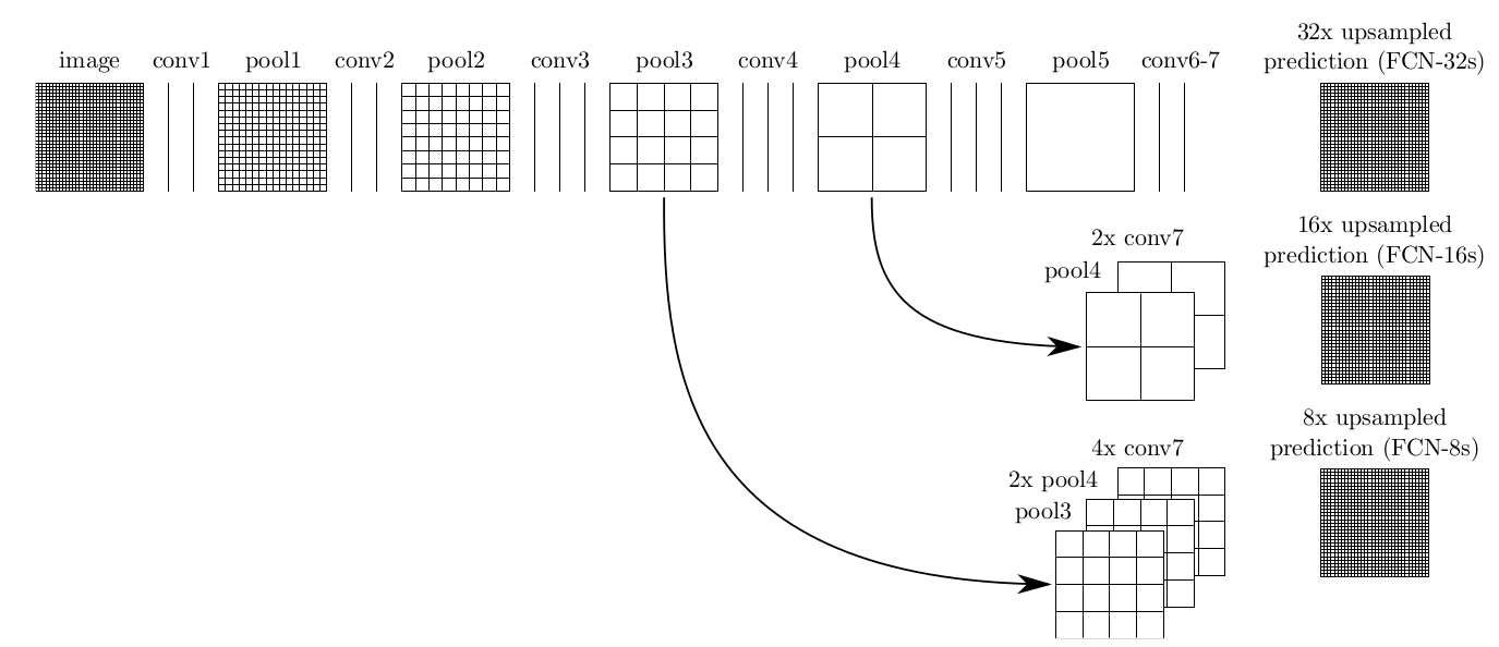
But the output segmented image is not accurate enough compared to the ground truth, and it is known, after pass through convolutional layers and pooling layers, the size of the image and also resolution is reduced. In order to increase the accuracy of image segmentation, coarse, high layer information are combined with fine, low layer information. So not only the output layer is upsampled, but also the pooling layers before, and the results is combined with the output layer, which shows a better performance. Pass through the original 5 convolutional and pooling layers of VGG network, the resolution of the image is reduced 2, 4, 8, 16, 32 times. For the last output image, it should be upsampled 32 times to be the same size as the input image (Figure 7). More details are summarized in the following table [1]:
- First row (FCN-32s): the single-stream net, upsamples stride 32 predictions back to pixels in a single step.
- Second row (FCN-16s): Combining predictions from both the final layer and the pool4 layer, at stride 16, lets the net predict finer details, while retaining high-level semantic information.
- Third row (FCN-8s): Additional predictions from pool3, at stride 8, provide further precision. Three upsampled ways are illustrated in the right figure, pooling and prediction layers are shown as grids that reveal relative spatial coarseness, while intermediate layers are shown as vertical lines.
The refined fully convolutional network is evaluated by the images from ImagNet, a example is illustrated in the (figure 8), from the left to the right are original images, output image from 32, 16,8 pixel stride nets and the ground truth. As you can see, the output image combine with pool4 layer is loser to the ground truth compared to FCN-32s and FCN-16s. The success of fully convolutional network for semantic segmentation can be summarized in the following table:
- Use the architecture of VGG network and the pre-trained weights and biases for first five convolutional layers as fine-tuning.
- Replace the fully connected layers by convolutional layers to solve dense prediction problem like image segmentation.
- Use deconvolutional layers to upsample the output image, make it same size as the input image, combine the information of pooling layers before to get better performance.


2 Kommentare
Unbekannter Benutzer (ga25ked) sagt:
31. Januar 2017In general, the explanation of the topic is good and it is easy to read.
Suggestions:
- link each paragraph to a source
- I think the bibliography style is inconsistent with the rest of the wiki
For example:
3. SegNet: A Deep Convolutional Encoder-Decoder Architecture for Robust Semantic Pixel-Wise Labelling
3. Badrinarayanan, Vijay, Ankur Handa, and Roberto Cipolla. "Segnet: A deep convolutional encoder-decoder architecture for robust semantic pixel-wise labelling." arXiv preprint arXiv:1505.07293 (2015).
Corrections:
truth compared to FCN-32s abd FCN-16s
truth compared to FCN-32s and FCN-16s
I can’t say much more. Good work.
Unbekannter Benutzer (ga58zak) sagt:
31. Januar 2017thanks for your advice.
best
Bo