Abstract
In this blog the topic of Sensorless Ultrasound (US) Compounding shall be introduced. The problem statement shall be explained and current procedure and methods for 3D Ultrasound reconstruction will be discussed. We then plan to throw light upon how deep learning based methods are improving the whole process of reconstructing 3D Ultrasound images from 2D Ultrasound images. For this purpose two papers have been selected and reviewed thoroughly. Each paper highlights and discusses two different deep learning methods and approaches for 3D US reconstruction by compounding of 2D US images. We will also compare the two approaches and how well the papers are written as well.
Author: Devansh Sharma
Tutor: Mohammad Farid Azampour
1. Introduction
1.1 2D Ultrasound Imaging
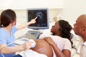
2D ultrasound imaging is a widely used medical technique that provides valuable insights into the human body. It utilizes high-frequency sound waves to generate real-time, two-dimensional images of organs, tissues, and developing fetuses. The procedure involves a transducer that emits sound waves, which then bounce back and are detected to create images. This non-invasive and safe imaging modality is particularly useful in obstetrics for monitoring fetal development, identifying potential abnormalities, and determining the gender of the baby. It also aids in diagnosing various conditions affecting internal organs, such as gallstones or kidney stones. 2D ultrasound imaging continues to play a crucial role in modern healthcare, providing valuable diagnostic information with minimal risk to patients.

Figure 1. Fetal Ultrasound [1]
1.2 3D Ultrasound Imaging
In recent years, the field of medical imaging has witnessed significant advancements, one of which is the development of 3D ultrasound image reconstruction methods. These techniques utilize a series of 2D ultrasound images to create a three-dimensional representation of the scanned area. By integrating multiple 2D images captured from different angles, the reconstructed 3D image provides a more comprehensive and detailed view of the internal structures.
To perform 3D ultrasound image reconstruction, specialized devices are used in practice. These devices consist of a transducer, which emits and receives ultrasound waves, and a computer system that processes the collected data. The transducer is maneuvered over the patient's body to capture a sequence of 2D images, covering the desired area from multiple perspectives. The computer then employs sophisticated algorithms to align and merge these images, constructing a coherent 3D representation.
This technology offers numerous benefits in various medical fields. In obstetrics, it enables healthcare professionals to visualize the fetus in three dimensions, aiding in the diagnosis of congenital anomalies and assisting in surgical planning. In cardiology, 3D ultrasound helps assess heart function and detect abnormalities. Additionally, it finds applications in abdominal imaging, urology, and musculoskeletal examinations.
The availability of 3D ultrasound image reconstruction has revolutionized diagnostic capabilities, providing clinicians with a powerful tool for improved visualization and accurate assessment of anatomical structures.
 Figure 2. 3D Ultrasound Imaging setup for spine imaging [2]
1.3 Problem Statement
Current 3D ultrasound image reconstruction methods face several significant challenges that hinder their widespread adoption and effectiveness. One major concern is the high cost associated with external tracking approaches, making them financially prohibitive for many healthcare facilities. Moreover, these methods often have limited use cases, restricting their applicability in various medical scenarios. Additionally, the sensors utilized in external tracking systems are prone to errors, leading to inaccuracies in the reconstructed 3D images.
Optical tracking methods encounter occlusion problems, where certain areas of the scanned object are obscured from the tracking system's view, resulting in incomplete reconstructions. Electromagnetic tracking devices, on the other hand, suffer from interference issues, affecting the reliability and precision of the reconstructed images.
Conventional methods like Voxel-based Nearest Neighbour (VNN) lack the necessary efficiency and accuracy required for precise 3D image reconstructions. Even image processing methods, while promising, still need improvement to overcome various artifacts and limitations inherent in current techniques. Addressing these challenges is crucial to enhance the overall performance and applicability of 3D ultrasound image reconstruction, allowing for better diagnostic capabilities and more informed medical decision-making.
1.4 Deep Learning Solutions
Deep learning methods have made significant contributions to improving the performance and process of 3D ultrasound image reconstruction. One notable example is the DCL-Net (Deep Convolutional Level-set Network), which leverages deep convolutional neural networks (CNNs) and level-set-based contour evolution. DCL-Net has demonstrated promising results by effectively reconstructing volumetric images from 2D ultrasound slices. It combines the power of CNNs to extract meaningful features from the input images with contour evolution techniques to refine the contour and generate accurate 3D reconstructions.
Another noteworthy advancement in this field is the use of NeRF (Neural Radiance Fields) based methods. NeRF is a novel approach that represents the volumetric scene as a continuous function, allowing for high-quality 3D reconstruction from sparse and unstructured data. By training deep neural networks on a large dataset of 2D ultrasound images, NeRF-based methods can estimate the radiance and geometry of the scene, enabling the generation of detailed and realistic 3D reconstructions.
These deep learning-based solutions have improved the overall performance of 3D ultrasound image reconstruction by addressing limitations such as artifacts, inaccuracies, and the need for manual intervention. They offer the potential for more accurate, efficient, and automated reconstruction processes, enhancing the diagnostic capabilities of ultrasound imaging in various medical applications. Continued research and development in deep learning methods, including DCL-Net and NeRF-based approaches, hold promise for further advancements in 3D ultrasound image reconstruction, leading to improved healthcare outcomes and patient care.

Figure 3. An overview of the proposed DCL-Net, which takes one video segment as input
volume and gives the mean motion vector as the output [3]
Methodology and Evaluation
Now we look at two different papers and throw light on their methodology. We will also try to explain them in bit more detail and highlight the experiments conducted and final results obtained.
2.1 NeRF based Implicit Representation Method for Freehand 3D Ultrasound Image Reconstruction
Motivations
The motivation of this research paper is to address the limitations and artifacts in 3D ultrasound reconstruction of the carotid artery. The authors highlight that carotid atherosclerosis (CA) is a prevalent condition with significant health implications, including stroke, and ultrasound imaging is commonly used for clinical examination due to its non-invasiveness and cost-effectiveness. However, current ultrasound methods only provide 2D information and rely heavily on the sonographer's experience.
To overcome these limitations, the authors propose the development of a novel 3D ultrasound reconstruction algorithm based on deep learning. The objective is to improve the image quality of the reconstructed volume and reduce artifacts. The authors mention that traditional methods, such as voxel-based nearest neighbor (VNN), have been commonly used but may not provide satisfactory results.
Method Overview
NeRF - Neural Radiance Fields
The method used is based on NeRF (Neural Radiance Field) which is a cutting-edge computer vision method that reconstructs scenes and synthesizes novel views using deep learning. It models a scene as a continuous function mapping 3D coordinates to radiance values. By training a neural network on image and pose data, NeRF generates highly realistic views from any viewpoint, capturing fine details and lighting effects. While computationally demanding, NeRF's advancements have led to optimizations for real-world applications. This technique has the potential to revolutionize virtual reality, video game design, and other fields reliant on accurate scene reconstruction and rendering.

Figure 4. An Overview of NeRF scene representation [4]
Data acquisition and pre processing
The authors acquired 15 original datasets from a local hospital using a portable freehand 3D ultrasound imaging system. These datasets were obtained from clinical sources, rather than being created by the authors themselves. The datasets consisted of 2D transverse images captured using a 10-MHz linear array transducer and corresponding location information obtained from an electromagnetic tracker. Each dataset contained 208 +- 46 transverse frames.
The authors then performed data acquisition and preprocessing on these 15 datasets as part of their research. The acquired 2D images were input into a segmentation neural network to obtain the semantic probabilistic distribution. Subsequently, the outputs from the neural network, along with the original images, were used for reconstructing the 3D volume. In addition, the authors also reconstructed the obtained data using the voxel-based nearest neighbor (VNN) method for comparison purposes.

Figure 5. Overall pipeline for data acquisition and processing [5]
Network architecture and training process
The method proposed in this research paper involves a deep learning architecture for reconstructing image volumes based on the neural radiance field (NeRF) approach. The objective is to jointly encode volume intensity and semantic features for improved reconstruction quality.
The neural network architecture is designed to map a 3D coordinate x to an output y, which consists of a semantic vector s and volume intensity i. The mapping function is represented as y = F _\theta(X) , where F_\theta is the learned neural network with its weights \theta. Position Encoding (PE) is utilized to map each 3D coordinate x to a higher-dimensional space, preserving high-frequency information of the volume intensity.
The network architecture is based on a multi-layer perceptron (MLP) from NeRF. The front layers are shared since semantic information and volume intensity are considered correlated. The width of the network is reduced before the outputs to separately output the semantic distribution and volume intensity. The SIREN activation function is applied to better represent the high-frequency domain. Connecting PE to the middle layer of the MLP aims to improve the quality of the reconstructed volume.
The entire network is trained from scratch using volume intensity loss L_i and semantic loss L_s. The volume intensity loss measures the difference between the predicted intensity and the ground truth, while the semantic loss measures the discrepancy between the predicted and ground truth semantic probabilities. The training loss combines both losses. Hence the final loss is L = L_i + L_s

Figure 6. The networks architecture. Locations were fed into networks after position encoding (PE). Volume intensity (i) and semantic (s) probability were the functions of 3D locations. [5]
Experiments and Conclusions
Evaluation metrics
The evaluation metrics used in this paper to assess the image quality of the reconstructed volume are discontinuity, curvature, and distortion. These metrics are calculated on the transverse frames of the volume.
Discontinuity: This metric characterizes break points in the region of interest (ROI). If the voxels from the vessel wall in a frame are not connected, that frame is marked as discontinuity.
Curvature: Curvature is calculated from the outer edge of vessel walls on non-discontinuous frames. The curvature of a voxel is approximated by its nearest adjacent voxels. For a voxel V_{out} ,the adjacent voxels were defined as V_{adj} \in \{ V_{out-N}, V_{out-N+1}, ....V_{out +N}\} . Therefore, the curvature at V_{out} could be defined as: Curvature(V_{out}) = median(\{f_c(V_{out-1},V_{out},V_{out+1}), ... , f_c(V_{out-N}, V_{out} , V_{out+N})\})
The curvature at a voxel is determined by measuring the variance of curvatures along the edge. A smaller variance indicates a smoother boundary shape.Distortion: Distortion is calculated based on curvature. A predetermined threshold, C_{threshold}, is used, and if the curvature of a voxel exceeds this threshold, it is counted as a distortion point. In this study, C_{threshold} was set to 0.4.More distortion points indicate a more irregular shape of the vessel boundary.
To evaluate the image quality of the reconstructed volume, these metrics provide quantitative measures related to the continuity, smoothness, and regularity of the vessel wall.
Results
So having defined the evaluation metrics lets see the results of the experiments we obtained after training our model several times. So now lets see some visual comparisons that show improvement by using this method compared to a standard VNN on our dataset.
Figure 7 provides a visual comparison between the conventional VNN method and our proposed method. In the example image, a noticeable artifact is observed on the outer vessel wall in the VNN volume, as indicated by the white box. However, the new method successfully rectifies this discontinuity at the same position in the frame, resulting in a more coherent image. The green and red parts of the image are the segmented vessel wall area and lumen area respectively. The white box illustrates the position of discontinuity and its corresponding position on the image from our method.

Figure 7. Illustration of discontinuity rectification: a) the image with discontinuity from the VNN method; and b) the improved image from the new method. [5]
Figure 8 demonstrates an example of distortion in the outer edge of the vessel wall. The top edge appears rugged using the VNN method, whereas the new approach significantly smoothens the bumpy contour. The green and red parts of the image are the segmented vessel wall area and lumen area respectively. The white box illustrates the position of discontinuity and its corresponding position on the image from our method.

Figure 8. Illustration of distortion rectification: a) image from the VNN method; and b) image from the new method. [5]
Figure 9 showcases an example of a reconstructed 3D image. The green area represents the reconstructed tunica externa, and the red area indicates the lumen. Notably, our method yields a smoother reconstructed surface compared to the VNN method.

Figure 9. Illustration of 3D reconstructed volume: a) volume from the VNN method; and b) volume from the new method [5]
Furthermore, in Figure 6, a comparison of distortion numbers for one dataset illustrates that the new method reduces distortion in the majority of frames.
Table I [5] presents statistical results across all fifteen subjects, categorizing the cases as improved, unchanged, or deteriorated based on discontinuity, distortion, and variation of curvature. Significantly, almost two-thirds of the cases demonstrate improvement with method. The new approach particularly excels in reducing discontinuity and variation, surpassing its performance in reducing distortion.


Table II [5] provides quantitative differences for all improved cases. It highlights that our method consistently reduces artifacts by more than 30% across all evaluated categories.
In Table I we can see that there were 5 deteriorated cases in the experiments due to increased number of distortions. Training a Multi-Layer Perceptron (MLP) with high entropy may result in irregular boundaries and more distortion points compared to the conventional VNN method. Another factor that could contribute to these issues is the large gap between original image frames, which prevents the MLP from effectively filling the gap with appropriate semantic distributions, leading to additional distortions. To address these deteriorated cases, an alternative approach could involve utilizing semantic probability distribution to construct graphs and applying a graph-cut algorithm to refine the segmentation edge boundaries.

Figure 10. Comparison of distortion number from one dataset between VNN and the new method. [5]
In conclusion, the experiments demonstrate the superior performance of the new proposed method in reducing artifacts, such as discontinuity and distortion, resulting in smoother and more accurate vessel structures. These findings have significant implications for enhancing the diagnosis of carotid atherosclerosis (CA). Overall, our study presents a promising approach to improving 3D ultrasound reconstruction for carotid artery imaging. The proposed method demonstrated potential for more accurate diagnosis of carotid atherosclerosis (CA). However, there were a few deteriorated cases due to uncertainties in semantic segmentation and large gaps between image frames. Future work may involve refining the segmentation edge using graph-cut algorithms and validating the diagnostic results with additional and larger clinical data. Overall, this research presents a promising approach for enhancing 3D ultrasound reconstruction for carotid artery imaging.
2.2 Spatial Position Estimation Method for 3D Ultrasound Reconstruction Based On Hybrid Transformers
Motivations
The motivation for writing the paper and inventing this new transformer based method is to overcome the limitations and challenges of existing 3D US reconstruction methods, such as:
- The high cost, occlusion and interference problems of external tracking systems and markers
- The edge wave effect and low accuracy of speckle-based pose regression methods
- The lack of global spatial and positional information in CNN-based methods
- The cumulative error of ultrasound images in the reconstruction process
The authors aim to propose a novel hybrid transformer structure that can combine the local information extraction and the long-range information to improve the efficiency and accuracy of 3D US reconstruction.
Method Overview
Dataset preparation
In this paper, the researchers used two datasets: the human forearm dataset and a clinical dataset. The data collection was conducted with the approval of the local Institutional Review Board (IRB), ensuring ethical considerations.
Ultrasound images were acquired using a Mindray DC 6E Ⅱ ultrasound equipment with B-mode, capturing images at a rate of 60 frames per second. To determine the real spatial poses of the ultrasound probe during training, an optical marker and an NDI Polaris Vicra system were employed. The probes were calibrated in terms of spatial and temporal aspects using the Plus Toolkit.
The forearm dataset consisted of 100 cases, where the ultrasound probe had a movement range of 10-20 cm. On the other hand, the clinical dataset included 160 cases with a probe movement range of 15-25 cm. The clinical dataset had variable models and targets for data collection.
Each case in both datasets comprised 200 frames, with each frame having a size of 224×224 pixels. The researchers split the dataset into training, validation, and testing sets in a ratio of 3:1:1, respectively.
Method implementation

Figure 10. An overview of the proposed structure with a continuous ultrasound image frame sequence as input [6]
The authors propose a novel deep learning method for 3D ultrasound (US) reconstruction from 2D image sequences. The method consists of four main steps: add more math eqns here
- Local feature extraction and enhancement: The first step is to extract local information within the US image, such as the shape and texture of the tissues. The method uses a convolutional neural network (CNN) backbone to extract latent features from each US image and concatenate them into a feature sequence. The method also uses a difference map between adjacent images to enhance the local information. The difference map shows the changes in the image features over time, which can help to track the movement of the probe and the tissues. The image features are embedded into feature patches as such: Z_0 = B(S) + B(I_{diff}) = B[I_1;I_2;I_3; .... I_n] + B(I_{diff}) where B is our CNN backbone model, and image sequence S with frames as I_i \in \mathbf{R}^{W \times H \times C} where W,H and C represents resolution and channel of the image.
- Temporal transformer with IMU embedding: The second step is to capture global information among the US image sequence, such as the spatial and temporal relationships between different frames. The method uses a transformer structure to capture global dependencies among the feature sequence. The transformer is a type of neural network that can learn to attend to different parts of the input based on their relevance and importance. The method also incorporates the orientation information from an inertial measurement unit (IMU) as a priori information to embed the features. The IMU is a device that can measure the rotation and acceleration of the probe, which can provide relative positional information of the US images. We can represent the procedure of combining positional embedding and IMU info as such mathematically: Z_1 = Z_0 + E_{pos} hence now our output sequence is Z_1 \in \mathbf{R}^{d \times N} we can now embed IMU info after a MLP. Hence, E_{IMU} = MLP(R), E_{IMU} \in \mathbf{R}^{d \times N} now Z_2 = Z_1 + E_{IMU}.
- Multi-head self attention(MSA): The third step is to model the location information from different subspaces using multiple attention heads. The attention heads are parts of the transformer that can focus on different aspects of the input, such as shape, texture, motion, etc. The method uses multiple attention heads to model location information from different subspaces and combine them into a final output. This way, the method can capture more diverse and comprehensive information from the US image sequence. The transformer encoder has L layers and in each layer the MSA is connected and applied with Layer Norm (LN). We can show our structure output as given the previous embedded feature Z_2 as such:
Z^'_l = MSA(LN(Z_{l-1})) + Z_{l-1}, l = 1,2 ....L \\ Z_l = MLP(LN(Z_l)) + Z^'_l, l = 1,2 ....L \\ Y = LN(Z^'_l)
- Regression head: The fourth step is to predict the relative pose between adjacent images in the sequence, which is essential for 3D US reconstruction. The relative pose is a 6-degree-of-freedom (DoF) vector that describes the translation and rotation between two images. The method uses a regression layer to predict the relative pose between adjacent images in the sequence, based on the output of the multi-head self attention. Our output from transformer is so Y \in \mathbf{R}^{d \times N} and after regression head is Y \in \mathbf{R}^{6}
- Loss function: The final step is to measure the error between the predicted relative pose and the ground truth. The ground truth is the actual relative pose between two images, which can be obtained from external tracking systems or markers. The method uses the mean squared error (MSE) as the loss function, which calculates the average of the squared differences between the predicted and the ground truth values.
Experiments and Conclusions
To quantitatively compare our results with previous methods, we employed two commonly used evaluation metrics: final drift error and average distance error. The final drift error measures the distance between the center point of the initial and final frames in the labeled sequence and the predicted distance. This error reflects the cumulative inaccuracies in the reconstruction process. The average distance error, on the other hand, calculates the distance between corresponding corner points in each pair of frames throughout the entire sequence. This metric provides insights into the changes in orientation within the sequence. These evaluation indicators allow us to assess the accuracy and consistency of our method compared to existing approaches.

Figure 11. Results of comparison experiments and ablation experiments in forearm and clinical dataset. [6]
The results of comparison and ablation experiments can be seen in the above table. The forearm dataset results demonstrated the effectiveness of our proposed method compared to methods without the transformer encoder. Our hypothesis that the transformer encoder captures global information across long distances in ultrasound image sequences was validated. When considering the average distance error, our method outperformed the ResNet+ViT approach without IMU embedding, indicating that incorporating IMU information as prior pose knowledge effectively complemented the advantages of the transformer. Compared to the ViT model, our method achieved superior results due to its ability to extract local information in Max and Min cases. Additionally, it exhibited a 4.58% improvement and a 0.76mm reduction in final drift compared to ViT with direct image input, highlighting the effectiveness of combining local and global information.
Regarding the final drift results, the transformer encoder demonstrated a significant 25.84% improvement and a 5.52mm reduction in accuracy compared to the structure with CNN-I-O. It also outperformed the DCL-Net model with the same attention blocks, achieving a 6.49% improvement and a 1.10mm reduction. In the more challenging clinical dataset, the transformer-based model showed notable advancements in reducing cumulative errors compared to models that relied solely on local information extraction. The inclusion of IMU information further contributed to minimizing average distance errors. However, the utilization of difference maps to enhance sequence information did not have a significant impact on the results.

Figure 12. Results of feature map visualization of ultrasound images on sequence scale [6]
To help understand the role of the transformer in ultrasound (US) images, a visualization technique called attention maps based on [7] was employed. Unlike traditional methods that focus on local image information, the transformer captures long-range relationships within image sequences. To visualize this, we generated attention maps by overlaying them on the difference maps. The difference maps serve as a representation of the features at the sequence scale.
In Figure 12, the visualization results are presented. The highlighted regions in the attention maps corresponded to the difference parts of the difference maps. This correspondence indicated that the transformer learned a meaningful relationship between images within the sequence.
The significance of the transformer in this context becomes apparent through these visualizations. It enables the model to capture and analyze global information spanning multiple frames, allowing it to understand the spatial and temporal context of the US image sequence. By leveraging this long-range relationship modeling, the transformer empowers our method to make accurate predictions and reduce cumulative errors.

Table III. Comparison of the final drift obtained by different methods on image sequences with different length.


Figure 13. Comparison of the final drift obtained by different methods on image sequences with different lengths. Figure 14. Comparison of the reconstruction results.
To further demonstrate the advantages of the proposed method in capturing long-range information, they conducted evaluations on ultrasound (US) image sequences of varying lengths. The comparison results are presented in Figure 13. For sequences with a length of 50 frames, all the compared methods showed similar final drift error results. However, as the sequence length increased, USFormer, gradually outperformed the CNN-based methods. Notably, USFormer exhibited significant improvements in cases where the sequence length exceeded 100 frames. This indicated that the ability to capture global information effectively reduced cumulative errors in the reconstruction process. For specific quantitative results, please refer to Table III.
To qualitatively showcase the reconstruction performance, they selected four test cases with varying degrees of quality. These cases included the best, worst, and two medium-quality cases reconstructed using USFormer, along with comparisons to CNN, DCL-Net, and ground truth. Figure 14 illustrates these results. It can be observed that our proposed method outperformed the other approaches in terms of reducing final drift. However, it's important to note that even with the best method and the gold standard (ground truth), there were significant errors in reconstructing complex data from clinical scenarios. This may be attributed to the probe not moving strictly in a single direction during data collection, as the round-trip movements can introduce increased errors.
In conclusion, USFormer demonstrated superior reconstruction performance, particularly in capturing long-range information, compared to the CNN-based approaches. However, it is crucial to acknowledge the inherent challenges and limitations when dealing with complex clinical data, where various factors can contribute to errors in the reconstruction process. The paper proposes a method that combines local and global information within the image and further embeds IMU information to improve the accuracy of 3D ultrasound reconstruction. The method reduces the drift error in the reconstruction process compared to state-of-the-art methods. However, the paper’s dataset is limited in type and number. In future work, the authors plan to pay more attention to complex reconstruction in different US imaging targets and scanning procedures.
3. Comparison
Comparison between the two methods
| NeRF based method | Hybrid Transformer method |
|---|---|
| Focuses on Carotid artery and Carotid Atherosclerosis (CA) | More generalized approach |
| Utilizes NeRF , and has a more simple and effective approach | Utilizes transformers very well |
| Interesting Evaluation Metrics | Standard metrics and loss function |
| Improves over current practice and provides improvement ideas for future | Improves on previous deep learning and attention based architectures |
| Semantic segmentation information is utilized and clever data pre processing | Utilises CNN backbone first and IMU and Positional embedding later for transformer encoder input |
Strengths
| NeRF based method | Hybrid Transformer method |
|---|---|
| Concise writing | Clear explanation of method and experiments |
| More focused use case | More general approach |
| Practical and visual 3D results | Comparison with multiple methods |
| Attention to detail and novel architecture | Novel and complex architecture with clear structure |
Shortcomings
| NeRF based method | Hybrid Transformer method |
|---|---|
| Less data acquisition details, smaller dataset | Images and results visualization bit small and crowded |
| Only one method to compare i.e. VNN | Significant error in Clinical data |
| Difficult to understand some implementation and mathematical details | Dataset limited in type and number |
| No public data or code available | No public data or code available |
4. Review
During our discussion, we explored two distinct approaches to 3D ultrasound (US) reconstruction, which leverage advanced deep learning and computer vision techniques. These methods offer significant advantages by eliminating the requirement for precise and costly sensors typically used in traditional approaches. Notably, both methods demonstrated superior performance compared to the current state-of-the-art techniques in this field.
The first paper we examined showcased the potential of the proposed method to facilitate more accurate diagnoses of various medical conditions, particularly carotid atherosclerosis (CA). By harnessing deep learning and computer vision algorithms, this approach exhibited promising results, opening up avenues for future research with larger and more diverse clinical datasets. The utilization of this method holds great promise in enhancing the accuracy and reliability of CA diagnoses, potentially leading to improved patient outcomes.
In the second paper, we delved into a technique that effectively addressed the issue of drift error encountered in the reconstruction process. This novel approach, incorporating deep learning and computer vision methodologies, demonstrated significant success in minimizing or eliminating the drift error. Moreover, this breakthrough paves the way for future investigations exploring different ultrasound imaging targets and scanning procedures. By mitigating the impact of drift error, this method enhances the overall quality and precision of 3D ultrasound reconstructions, offering researchers and clinicians greater confidence in the acquired data.
Overall, these two research papers highlight the immense potential of deep learning and computer vision in revolutionizing 3D ultrasound reconstruction. These approaches not only alleviate the need for expensive sensors but also surpass the performance of existing state-of-the-art methods. Furthermore, they open up exciting prospects for future research, expanding the application of these techniques to various clinical scenarios and enabling more accurate diagnoses and improved medical interventions.
5. References
[1] https://www.fda.gov/files/ultrasoundpregnancy.jpg
[2] Purnama , Ketut & Wilkinson, Michael & Veldhuizen , Albert & Van Ooijen , Peter & Lubbers, Jaap & Burgerhof , Johannes & Sardjono , Tri & Verkerke , Gijbertus . (2010). A framework for human spine imaging using a freehand 3D ultrasound system. Technology and health care : official journal of the European Society for Engineering and Medicine. 18. 1 17. 10.3233/THC 2010 0565.
[3] Guo, H., Xu, S., Wood, B., Yan, P. (2020). Sensorless Freehand 3D Ultrasound Reconstruction via Deep Contextual Learning. In: , et al. Medical Image Computing and Computer Assisted Intervention – MICCAI 2020. MICCAI 2020. Lecture Notes in Computer Science(), vol 12263. Springer, Cham. https://doi.org/10.1007/978-3-030-59716-0_44
[4] Ben Mildenhall and Pratul P. Srinivasan and Matthew Tancik and Jonathan T. Barron and Ravi Ramamoorthi and Ren Ng, " NeRF : Representing Scenes as Neural Radiance Fields for View Synthesis", ECCV 2020, 2020
[5] S. Song, Y. Huang, J. Li, M. Chen and R. Zheng, "Development of Implicit Representation Method for Freehand 3D Ultrasound Ima g e Reconstruction of Carotid Vessel," 2022 IEEE International Ultrasonics Symposium (IUS), Venice, Italy, 2022, pp. 1 4, doi : 10.1109/
[6] G. Ning, H. Liang, L. Zhou, X. Zhang and H. Liao, "Spatial Position Estimation Method for 3D Ultrasound Reconstruction Based on Hybrid Transformers," 2022 IEEE 19th International Symposium on Biomedical Imaging (ISBI), Kolkata, India, 2022, pp. 1 5, doi : 10.1109/
[7] R.R. Selvaraju, M. Cogswell, A. Das, et al., “Grad-cam: Visual explanations from deep networks via gradient-based localization,” International Journal of Computer Vision, vol. 128, no. 2, pp. 336-35, Feb. 2020.