Infinite Element for the Hybrid Trefftz Method

Authors: Viola Li, Affan Kalkavan, Debjit Majumder

Supervisors: Mirjam Lainer

Introduction

Motivation & Objectives

In soil dynamics one often has infinitely large domains, whereas only a small part is of interest. In order to simulate these problems efficiently, special methods are needed where only the region of interest is considered and reflecting waves at the boundary has to be avoided. The objective of this project is to perform a numerical analysis of unbounded elastodynamic problems using the Hybrid Trefftz method and so-called infinite elements. In order to describe such problems reasonably, a few assumptions need to be considered in terms of the domain, geometry and loading. Then the governing differential equations can be derived and the final system of equations can be found using the Helmholtz decomposition and the Galerkin weighted residual method. After the introduction of the basic principle of the Hybrid Trefftz method, unbounded domains are considered, which can be solved using absorbing elements or infinite elements. Both approaches will be introduced and the procedure to find the modified system of equations will be explained. Finally, some results for both approaches will be presented, compared and analysed regarding their advantages, disadvantages and limits.

Problem Description

Assumptions

The analysis of dynamically loaded media is a complex problem and the following assumptions are adapted to simplify the analysis:

• Continuous distribution of matter inside the body without an empty space thereby justifying the continuum assumption
• Isotropic material properties
• The strains and displacements are assumed to be small which implies that the deformation caused by the loading has a negligible effect on the equilibrium of forces (geometric linearity)
• Linear relationship between stresses and strains (material linearity)
• Periodic load cases

Domain and Geometry

Figure 1: Example domain and boundary [1].

In Figure 1 a general scheme of a possible structure of interest is depicted. The domain is represented by the symbol $//<![CDATA[ \begin{array}{l}\mathrm{V}\end{array} //]]>$ and $//<![CDATA[ \begin{array}{l}\mathrm{\Gamma}\end{array} //]]>$ stands for the boundary of such a body. This boundary can be partitioned into two sections, $//<![CDATA[ \begin{array}{l}\mathrm{\Gamma_u}\end{array} //]]>$ and $//<![CDATA[ \begin{array}{l}\mathrm{\Gamma_{\sigma}}\end{array} //]]>$, which are complementary to each other and non overlapping and are called Dirichlet and Neumann boundaries respectively. Boundary displacements are prescribed on the former one while boundary tractions are given on the latter one. As a result, Dirichlet boundary conditions are also called displacement boundary conditions and Neumann boundary conditions are also called force boundary condition.

Governing Equations 

Any loaded structure can be described by using three main sets of equations. Namely, the equilibrium equations, the kinematic equations and the constitutive equations. These equations, along with certain prescribed boundary conditions and initial conditions, fully describe the behaviour of the loaded structure by forming a governing system of equations. The equations and the boundary and initial conditions are as follows:

Equilibrium equation: $//<![CDATA[ \begin{array}{l}\mathrm{\boldsymbol{Dσ}\,+ ω^2ρ\boldsymbol{u} + \boldsymbol{b} = 0}\end{array} //]]>$ in $//<![CDATA[ \begin{array}{l}V\end{array} //]]>$

where $//<![CDATA[ \begin{array}{l}\boldsymbol{D}\end{array} //]]>$ represents the differential operator matrix, $//<![CDATA[ \begin{array}{l}\boldsymbol{σ}\end{array} //]]>$ represents the engineering stress vector, $//<![CDATA[ \begin{array}{l}ω\end{array} //]]>$ is the circular frequency, $//<![CDATA[ \begin{array}{l}ρ\end{array} //]]>$ is the mass density, $//<![CDATA[ \begin{array}{l}\boldsymbol{u}\end{array} //]]>$ is the displacement vector and $//<![CDATA[ \begin{array}{l}\boldsymbol{b}\end{array} //]]>$ represents body forces.

Kinematic equation:$//<![CDATA[ \begin{array}{l}\mathrm{\boldsymbol{ε}\,= \boldsymbol{D}^∗\boldsymbol{u}}\end{array} //]]>$ in $//<![CDATA[ \begin{array}{l}V\end{array} //]]>$

where $//<![CDATA[ \begin{array}{l}\boldsymbol{ε}\end{array} //]]>$ represents strain vector, $//<![CDATA[ \begin{array}{l}\boldsymbol{D^*}\end{array} //]]>$ represents the differential kinematic operator which is the adjoint of $//<![CDATA[ \begin{array}{l}\boldsymbol{D}\end{array} //]]>$.

Constitutive equation: $//<![CDATA[ \begin{array}{l}\mathrm{\boldsymbol{σ}\,= \boldsymbol{kε}}\end{array} //]]>$ in $//<![CDATA[ \begin{array}{l}V\end{array} //]]>$

where $//<![CDATA[ \begin{array}{l}\boldsymbol{k}\end{array} //]]>$ denotes the material matrix.

Dirichlet boundary condition: $//<![CDATA[ \begin{array}{l}\mathrm{\boldsymbol{u}\,= \boldsymbol{u_{\Gamma}}}\end{array} //]]>$ _{in $//<![CDATA[ \begin{array}{l}Γ_u\end{array} //]]>$}

$//<![CDATA[ \begin{array}{l}\boldsymbol{u_{\Gamma}}\end{array} //]]>$ represents the vector of prescribed displacement components.

Neumann boundary condition: $//<![CDATA[ \begin{array}{l}\boldsymbol{t} = \boldsymbol{t_{\Gamma}}\end{array} //]]>$ in $//<![CDATA[ \begin{array}{l}Γ_σ\end{array} //]]>$

$//<![CDATA[ \begin{array}{l}\boldsymbol{t_{\Gamma}}\end{array} //]]>$ represents the vector of prescribed traction components.

Hybrid Trefftz Method

Basic concept

The Hybrid Trefftz method is one of the most important computational methods that attempts to unite the versatility of conventional finite elements with the accuracy and high convergence rate exhibited by the boundary solution approaches. The basic principle of the Hybrid Trefftz method is similar to the FEM: the domain is discretized using finite elements and certain fields are approximated by shape functions multiplied by unknown coefficients. The main difference is that the basis functions in the Hybrid Trefftz method have to satisfy the governing differential equations of the problem a priori and a finite number of such basis functions is combined, such that the resulting function approximates the prescribed boundary conditions.

Figure 2: Domain discretization into finite elements [1].

As shown in figure 2, in order to implement the Hybrid Trefftz method, the domain needs to be discretized using finite elements $//<![CDATA[ \begin{array}{l}V^e\end{array} //]]>$ with the displacement boundaries or the Dirichlet boundaries represented by $//<![CDATA[ \begin{array}{l}Γ_u^e\end{array} //]]>$ and force boundaries or Neumann boundaries represented by $//<![CDATA[ \begin{array}{l}Γ_σ^e\end{array} //]]>$. Inter-element boundaries shared by two elements are also added to the set of Dirichlet boundaries. Two independent fields are approximated in each element, thus also the name Hybrid Trefftz method. The first one is  the displacement field in the domain and the second one is the traction field which is approximated on the Dirichlet boundaries. The corresponding approximation basis functions are used to enforce the inter-element and boundary displacement continuity using a Galerkin technique. The domain approximation is constrained to satisfy the locally the governing differential equation. It is important to note that the concept of nodal interpolation known from conventional FEM is completely omitted in Hybrid trefftz method. The bases used to approximate both displacement field in the domain and traction field on the boundaries are hierarchical and the coefficients correspond no longer to nodal values but are rather generalized quantities.

Domain Approximation

According to the Hybrid Trefftz Method, the displacement field is approximated in the element domain $//<![CDATA[ \begin{array}{l}V_e\end{array} //]]>$ and is expressed as,

$//<![CDATA[ \begin{array}{l}\boldsymbol{u} = \boldsymbol{UX} + \boldsymbol{u_{0}}\end{array} //]]>$

The matrix $//<![CDATA[ \begin{array}{l}\boldsymbol{U}\end{array} //]]>$ represents the basis functions, $//<![CDATA[ \begin{array}{l}\boldsymbol{X}\end{array} //]]>$ is vector of unknown coefficients, also called generalized displacements and $//<![CDATA[ \begin{array}{l}\boldsymbol{u_0}\end{array} //]]>$ represents the particular solution vector. The bases collected in matrix $//<![CDATA[ \begin{array}{l}\boldsymbol{U}\end{array} //]]>$ is constrained to satisfy the homogeneous part of the spectral Lamé equation, which is expressed as

$//<![CDATA[ \begin{array}{l}(λ + µ)\boldsymbol{∇∇^Tu} + µ\boldsymbol{∇}^2\boldsymbol{u} + ω^2ρ\boldsymbol{u} = 0\end{array} //]]>$

where $//<![CDATA[ \begin{array}{l}λ\end{array} //]]>$ and $//<![CDATA[ \begin{array}{l}µ\end{array} //]]>$ are Lamé parameters. 

The strain approximation basis can be directly estimated from the kinematic equation in terms of the displacement approximation basis as follows:

$//<![CDATA[ \begin{array}{l}\boldsymbol{ε} = \boldsymbol{D^*u} = \boldsymbol{D^*UX} + \boldsymbol{D^*u_{0}} = \boldsymbol{EX} + \boldsymbol{ε_{0}}\end{array} //]]>$ where $//<![CDATA[ \begin{array}{l}\boldsymbol{D^*U} = \boldsymbol{E}\end{array} //]]>$ and $//<![CDATA[ \begin{array}{l}\boldsymbol{D^*u_{0}} = \boldsymbol{ε_{0}}\end{array} //]]>$

Here $//<![CDATA[ \begin{array}{l}\boldsymbol{E}\end{array} //]]>$ is called the strain approximation basis.

Thus to construct the displacement basis $//<![CDATA[ \begin{array}{l}\boldsymbol{U}\end{array} //]]>$ and subsequently the strain basis $//<![CDATA[ \begin{array}{l}\boldsymbol{E}\end{array} //]]>$ it is necessary to solve the homogeneous part of the spectral Lamé equation.

Solution of the Homogeneous Spectral Lamé Equation

The homogeneous spectral Lamé equation is represented by

$//<![CDATA[ \begin{array}{l}(λ + µ)\boldsymbol{∇∇^Tu} + µ\boldsymbol{∇}^2\boldsymbol{u} + ω^2ρ\boldsymbol{u} = 0\end{array} //]]>$.

Application of the Helmholtz decomposition to the above equation allows to decouple the equation and to solve the dilatational and shear part separately. This leads to the following Helmholtz equations:

$//<![CDATA[ \begin{array}{l}\boldsymbol{∇}^2Φ_{p} + k_{p}^2Φ_{p} = 0\end{array} //]]>$ and $//<![CDATA[ \begin{array}{l}\boldsymbol{∇}^2Φ_{s} + k_{s}^2Φ_{s} = 0\end{array} //]]>$

where $//<![CDATA[ \begin{array}{l}k_p\end{array} //]]>$ and $//<![CDATA[ \begin{array}{l}k_s\end{array} //]]>$ represent the wave numbers of p-waves and s-waves respectively and $//<![CDATA[ \begin{array}{l}Φ_{p}\end{array} //]]>$ and $//<![CDATA[ \begin{array}{l}Φ_{s}\end{array} //]]>$ represent the dilatational and shear potential respectively. Also $//<![CDATA[ \begin{array}{l}k_p\end{array} //]]>$ and $//<![CDATA[ \begin{array}{l}k_s\end{array} //]]>$ can be represented in terms of p-wave velocity $//<![CDATA[ \begin{array}{l}c_p\end{array} //]]>$ and s-wave velocity $//<![CDATA[ \begin{array}{l}c_s\end{array} //]]>$ as follows,

$//<![CDATA[ \begin{array}{l}k_p = \frac{ω}{c_p}\end{array} //]]>$ and $//<![CDATA[ \begin{array}{l}k_s = \frac{ω}{c_s}\end{array} //]]>$

Using the ansatz

$//<![CDATA[ \begin{array}{l}Φ_{α,n} = W_{n}(k_{α}r)exp(inθ)\end{array} //]]>$,

where $//<![CDATA[ \begin{array}{l}α = (p,s)\end{array} //]]>$ and $//<![CDATA[ \begin{array}{l}r\end{array} //]]>$ and $//<![CDATA[ \begin{array}{l}θ\end{array} //]]>$ are the radial and angular coordinates, we will eventually arrive at the Bessel equation which is defined as follows:

$//<![CDATA[ \begin{array}{l}\frac{\partial^2 W_{n}(ζ)}{\partial ζ^2} + \frac{1}{ζ}\frac{\partial W_{n}(ζ)}{\partial ζ} + (1 - \frac{n^2}{ζ^2})W_{n}(ζ) = 0\end{array} //]]>$ where $//<![CDATA[ \begin{array}{l}ζ = k_{α}r\end{array} //]]>$.

For each integer $//<![CDATA[ \begin{array}{l}n\end{array} //]]>$, there exists two linearly independent solutions as the Bessel equation is a second order linear differential equation. Various formulations of these linearly independent pairs may be adopted. In this project the Hankel functions of first and second kind are considered for the representation of the solutions of $//<![CDATA[ \begin{array}{l}W_n(ζ)\end{array} //]]>$ and are represented as $//<![CDATA[ \begin{array}{l}H_n^(^1^)(ζ)\end{array} //]]>$ and $//<![CDATA[ \begin{array}{l}H_n^(^2^)(ζ)\end{array} //]]>$ respectively. The Hankel functions can be represented in terms of the first and second kind of Bessel function, which are represented by $//<![CDATA[ \begin{array}{l}J_n\end{array} //]]>$ and $//<![CDATA[ \begin{array}{l}Y_n\end{array} //]]>$ respectively, as follows;

$//<![CDATA[ \begin{array}{l}H^(^1^)_{n}(ζ) = J_{n}(ζ) + iY_{n}(ζ) & and & H^(^2 ^)_{n}(ζ) = J_{n}(ζ) - iY_{n}(ζ)\end{array} //]]>$

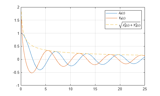
Figure 3: Real and imaginary part of the Hankel function of second kind and order zero [2].

Figure 3 shows the Hankel function of first kind and order zero. The real and imaginary parts of the function correspond to the Bessel functions of first and second kind. The absolute values reveal the asymptotic behavior of Hankel functions. Hankel functions are singular at the origin. It is therefore important to place the origin of the reference system outside of the analysed elements when using Hankel functions in the approximation basis. In the examples that we analysed, we used a global reference system, where the origin for every element is located at $//<![CDATA[ \begin{array}{l}(0,0)\end{array} //]]>$. The elements are then placed at a certain distance $//<![CDATA[ \begin{array}{l}r_{min}\end{array} //]]>$ to the origin.

For a single order $//<![CDATA[ \begin{array}{l}n\end{array} //]]>$, the unknown dilatational and shear potential can thus be expressed as

$//<![CDATA[ \begin{array}{l}Φ_{p,n} = W_n(k_pr)exp(inθ) & and & Φ_{s,n} = W_n(k_sr)exp(inθ)\end{array} //]]>$.

There is an infinite number of functions satisfying the Helmholtz equations and the complete solution can be expressed as a linear combination of all terms as

$//<![CDATA[ \begin{array}{l}Φ_p = \sum_{n = -{\infty}}^{n = {\infty}}c_p_,_nΦ_p_,_n & and & Φ_s = \sum_{n = -{\infty}}^{n = {\infty}}c_s_,_nΦ_s_,_n\end{array} //]]>$.

Thus the displacement is given by

$//<![CDATA[ \begin{array}{l}\boldsymbol{u} = \boldsymbol{∇}Φ_p + \boldsymbol{\tilde{∇}}Φ_s= \sum_{n = -{\infty}}^{n = {\infty}}c_p_,_n\boldsymbol{∇}Φ_p_,_n + c_s_,_n\boldsymbol{\tilde{∇}}Φ_s_,_n\end{array} //]]>$.

Domain Approximation Basis

The displacement field can be decomposed into dilatational and shear potentials using Helmholtz decomposition. As a result individual modes in the basis $//<![CDATA[ \begin{array}{l}\boldsymbol{U}\end{array} //]]>$ can also be separated into two components. Therefore, for a single order $//<![CDATA[ \begin{array}{l}n\end{array} //]]>$, a submatrix $//<![CDATA[ \begin{array}{l}\boldsymbol{U_n}\end{array} //]]>$ collects two different basis functions,one for each of the displacement components and has the following form:

$//<![CDATA[ \begin{array}{l}\boldsymbol{U_n} = \begin{bmatrix}\boldsymbol{∇}Φ_{p,n} & \boldsymbol{\tilde{∇}}Φ_{s,n}\end{bmatrix} = \begin{bmatrix}\boldsymbol{ ∇}W_n(k_pr)exp(inθ) & \boldsymbol{\tilde{∇}}W_n(k_sr)exp(inθ)}\end{bmatrix}\end{array} //]]>$

In $//<![CDATA[ \begin{array}{l}\boldsymbol{U}\end{array} //]]>$ the first column contains the dilatational part and the second column contains the shear part. Now these individual basis functions are combined to form the complete basis $//<![CDATA[ \begin{array}{l}\boldsymbol{U}\end{array} //]]>$ for order $//<![CDATA[ \begin{array}{l}-N< n< N\end{array} //]]>$ where $//<![CDATA[ \begin{array}{l}N\end{array} //]]>$ is the chosen maximum order of the function $//<![CDATA[ \begin{array}{l}W_n\end{array} //]]>$ with $//<![CDATA[ \begin{array}{l}2N + 1\end{array} //]]>$ sub-matrices that includes a total of $//<![CDATA[ \begin{array}{l}2(2N+1)\end{array} //]]>$ approximation functions.The complete basis is shown below,

$//<![CDATA[ \begin{array}{l}\boldsymbol{U} = \begin{bmatrix}\boldsymbol{U_{-N}} ...... \boldsymbol{U_n} ...... \boldsymbol{U_N}\end{bmatrix}\end{array} //]]>$

As the number of terms in the complete basis increases the elements get richer but this comes with an additional cost of numerical issues. this is because at the vicinity of origin higher order Bessel functions take much smaller values compared to the lower order ones. Now in the problem that we have solved we have considered polar coordinates as our system because $//<![CDATA[ \begin{array}{l}Φ_{p,n}\end{array} //]]>$ and $//<![CDATA[ \begin{array}{l}Φ_{s,n}\end{array} //]]>$ directly depends on the radius $//<![CDATA[ \begin{array}{l}r\end{array} //]]>$ and angle$//<![CDATA[ \begin{array}{l}θ\end{array} //]]>$. In the polar form the $//<![CDATA[ \begin{array}{l}\boldsymbol{U_n}\end{array} //]]>$ matrix looks as follows,

$//<![CDATA[ \begin{array}{l}\boldsymbol{U_n} = \begin{bmatrix}\ \boldsymbol{∇}Φ_{p,n} & \boldsymbol{\tilde{∇}}Φ_{s,n}\end{bmatrix} = \begin{bmatrix}\cos{ θ} & -\sin{ θ}\\ \sin{ θ} & \cos{ θ}\end{bmatrix}\begin{bmatrix}\frac{\partial Φ_{p,n} }{\partial r} & \frac{1}{r}\frac{\partial Φ_{s,n} }{\partial r}\\\frac{1}{r}\frac{\partial Φ_{p,n} }{\partial r} & -\frac{\partial Φ_{s,n} }{\partial r}\end{bmatrix} = \boldsymbol{TU_n^{r,θ}}\end{array} //]]>$

In the above equation $//<![CDATA[ \begin{array}{l}\boldsymbol{T}\end{array} //]]>$ is the transformation matrix and $//<![CDATA[ \begin{array}{l}\boldsymbol{U_n^{r,θ}}\end{array} //]]>$ collects the basis functions in $//<![CDATA[ \begin{array}{l}r\end{array} //]]>$ and $//<![CDATA[ \begin{array}{l}θ\end{array} //]]>$ directions. Substituting the values of $//<![CDATA[ \begin{array}{l}Φ_{p,n}\end{array} //]]>$ and $//<![CDATA[ \begin{array}{l}Φ_{s,n}\end{array} //]]>$ in $//<![CDATA[ \begin{array}{l}\boldsymbol{U_n^{r,θ}}\end{array} //]]>$ will lead to more simplified form and that has been used by us in the matlab code to solve the problem of infinite element. After all the substitutions the $//<![CDATA[ \begin{array}{l}\boldsymbol{U_n^{r,θ}}\end{array} //]]>$ looks as follows,

$//<![CDATA[ \begin{array}{l}\boldsymbol{U_n^{r,θ}} = 0.5\begin{bmatrix}k_p(W_{n-1} - W_{n+1}) & ik_s(W_{n-1} + W_{n+1})\\ ik_p(W_{n-1} + W_{n+1}) & k_s(W_{n+1} - W_{n-1})\end{bmatrix}exp(inθ)\end{array} //]]>$

The corresponding strain field basis looks as follows,

$//<![CDATA[ \begin{array}{l}\boldsymbol{E_n} = \boldsymbol{D^*U_n} = \boldsymbol{T_εE_n^{r,θ}}\end{array} //]]>$

where $//<![CDATA[ \begin{array}{l}\boldsymbol{T_ε}\end{array} //]]>$ is the transformation matrix and $//<![CDATA[ \begin{array}{l}\boldsymbol{E_n^{r,θ}}\end{array} //]]>$ collects the basis functions in polar form.

$//<![CDATA[ \begin{array}{l}\boldsymbol{E_n^{r,θ}} = 0.25\begin{bmatrix}k_p^2(W_{n-2} - 2W_{n} + W_{n+2}) & ik_s^2(W_{n-2} - W_{n+2})\\ -k_p^2(W_{n-2} + 2W_{n} + W_{n+2}) & -ik_s^2(W_{n-2} - W_{n+2})\\ 2ik_p^2(W_{n-2} - W_{n+2}) & 2k_s^2(W_{n-2} + W_{n+2}) \end{bmatrix}exp(inθ)\end{array} //]]>$

From the ordering of the bases $//<![CDATA[ \begin{array}{l}\boldsymbol{U}\end{array} //]]>$ and $//<![CDATA[ \begin{array}{l}\boldsymbol{E}\end{array} //]]>$ also layout of the vector of unknown coefficients $//<![CDATA[ \begin{array}{l}\boldsymbol{X}\end{array} //]]>$ can be deduced. It can be visualized as,

$//<![CDATA[ \begin{array}{l}\boldsymbol{X} = \begin{bmatrix}\boldsymbol{ X_{-N}}......\boldsymbol{X}_n......\boldsymbol{X_N}\end{bmatrix}^\boldsymbol{T} = \begin{bmatrix} \boldsymbol{X_{-N}^p}} & \boldsymbol{X_{-N}^s}......\boldsymbol{X_n^p} &\boldsymbol{ X_n^s}......\boldsymbol{X_N^p} &\boldsymbol{ X_N^s}\end{bmatrix}^\boldsymbol{T}\end{array} //]]>$

Boundary Approximation

The second field that is to be approximated are the boundary tractions on the Dirichlet boundaries $//<![CDATA[ \begin{array}{l}Γ_u^e\end{array} //]]>$. These boundaries not only mean the external boundaries but also the inter-element boundaries where displacement continuity has to be enforced. The relation reads as follows,

$//<![CDATA[ \begin{array}{l}\boldsymbol{t} = \boldsymbol{Zp}& on & Γ_{u}^e\end{array} //]]>$

where $//<![CDATA[ \begin{array}{l}\boldsymbol{Z}\end{array} //]]>$contains the boundary approximation basis,  $//<![CDATA[ \begin{array}{l}\boldsymbol{p}\end{array} //]]>$ stands for vector of unknown coefficients or generalized tractions. Chebyshev polynomials of type I are adopted for the basis $//<![CDATA[ \begin{array}{l}\boldsymbol{Z}\end{array} //]]>$. They are defined for a side coordinate $//<![CDATA[ \begin{array}{l}ξ ∈ (-1,1)\end{array} //]]>$,

$//<![CDATA[ \begin{array}{l}Z_m(ξ) = \cos{(m\cos^{-1}{ξ})}\end{array} //]]>$

where $//<![CDATA[ \begin{array}{l}m = 0,1,2,....,M\end{array} //]]>$ denotes the order of the polynomial. The first four basis functions are depicted in figure 4.

Figure 4: Traction approximation basis functions of different orders [1].

The indvidual components are then ordered in complete matrix $//<![CDATA[ \begin{array}{l}\boldsymbol{Z}\end{array} //]]>$ as

$//<![CDATA[ \begin{array}{l}\boldsymbol{Z} = \begin{bmatrix}\boldsymbol{Z_v }& 0\\0 &\boldsymbol{ Z_v}\end{bmatrix}\end{array} //]]>$,

where $//<![CDATA[ \begin{array}{l}\boldsymbol{Z_v} = \begin{bmatrix}Z_0 & Z_1......Z_M\end{bmatrix}\end{array} //]]>$. Consequently the vector for generalized tractions is

$//<![CDATA[ \begin{array}{l}\boldsymbol{p} = \begin{bmatrix}\boldsymbol{p_x^T} &\boldsymbol{ p_y^T}\end{bmatrix}^\boldsymbol{T}\end{array} //]]>$.

The traction vector $//<![CDATA[ \begin{array}{l}\boldsymbol{t(x,y)}\end{array} //]]>$ is a function of Cartesian coordinates, however, the approximation basis $//<![CDATA[ \begin{array}{l}Z(ξ)\end{array} //]]>$ is a function of the local edge coordinate $//<![CDATA[ \begin{array}{l}ξ ∈ (-1,1)\end{array} //]]>$. Therefore, for every Dirichlet edge, there must exist a function $//<![CDATA[ \begin{array}{l}h(ξ)\end{array} //]]>$ mapping the coordinate $//<![CDATA[ \begin{array}{l}ξ\end{array} //]]>$ to Cartesian coordinates $//<![CDATA[ \begin{array}{l}\begin{bmatrix} \boldsymbol{x} & \boldsymbol{y}\end{bmatrix}^\boldsymbol{T}\end{array} //]]>$.
.

Governing System

The Galerkin weighted residual method is generally used to derive the finite element system of equation. Firstly, the equilibrium equations are implemented in their weak form and  substitution of the material law and the kinematic equation is done. This leads to the first set of finite element equations.

If we define

$//<![CDATA[ \begin{array}{l}\boldsymbol{D} =\int\boldsymbol{\hat{U}}^T\boldsymbol{NkE}d\Gamma^{e}\end{array} //]]>$

where matrix $//<![CDATA[ \begin{array}{l}\boldsymbol{N}\end{array} //]]>$ collects the component of outward normal at the boundary.

$//<![CDATA[ \begin{array}{l}\boldsymbol{B} =\int\boldsymbol{\hat{U}}^T\boldsymbol{Z}d\Gamma_u^{e}\end{array} //]]>$

$//<![CDATA[ \begin{array}{l}\boldsymbol{\overline{t_\Gamma}} =\int\boldsymbol{\hat{U}}^T\boldsymbol{t_\Gamma}d\Gamma_\sigma^{e}\end{array} //]]>$

$//<![CDATA[ \begin{array}{l}\boldsymbol{\overline{t_{\Gamma}_0}} =\int\boldsymbol{\hat{U}}^T\boldsymbol{Nkε_0}d\Gamma^{e}\end{array} //]]>$

Then the equilibrium equation is,

$//<![CDATA[ \begin{array}{l}\boldsymbol{DX - Bp} =\boldsymbol{\overline{t_\Gamma} - \overline{t_{\Gamma}_0}}\end{array} //]]>$

Now in order to arrive at the second set of finite element equation Dirichlet's boundary condition and continuity equations are implemented in their weak form and are combined.

Now if we define

$//<![CDATA[ \begin{array}{l}\boldsymbol{\overline{u_\Gamma}} =\int\boldsymbol{Z}^T\boldsymbol{u_\Gamma}d\Gamma_u^{e}\end{array} //]]>$

$//<![CDATA[ \begin{array}{l}\boldsymbol{\overline{u_{\Gamma}_0}} =\int\boldsymbol{Z}^T\boldsymbol{u_0}d\Gamma_u^{e}\end{array} //]]>$

Then the equation can be written in its compact form in the following way,

$//<![CDATA[ \begin{array}{l}\boldsymbol{-\hat{B}^TX} = \boldsymbol{\overline{u_{\Gamma}_0}} - \boldsymbol{\overline{u_\Gamma}}\end{array} //]]>$

Thus combining the above two sets of finite element equation will lead to the governing system of equations which is mentioned below.

$//<![CDATA[ \begin{array}{l}\begin{bmatrix} \boldsymbol{D} & -\boldsymbol{B}\\ -\boldsymbol{\hat{B}}^T & \boldsymbol{0} \end{bmatrix} \begin{bmatrix} \boldsymbol{X}\\ \boldsymbol{p} \end{bmatrix} = \begin{bmatrix} \boldsymbol{\overline{t_{\Gamma}^{u}}}-\boldsymbol{\overline{t_{\Gamma_0}^{u}}}\\ \boldsymbol{\overline{u_{\Gamma_0}^{u}}}-\boldsymbol{\overline{u_{\Gamma}^{u}}} \end{bmatrix}\end{array} //]]>$

Hybrid Trefftz Method for Unbounded Problems

Sommerfeld Radiation condition

For unbounded domains the Sommerfeld radiation condition has to be fulfilled:

$//<![CDATA[ \begin{array}{l}\lim\limits_{r\to\infty} \left [\sqrt{k r}\left (\frac{\partial u}{\partial r}+ik u\right )\right ]=0\end{array} //]]>$,

where $//<![CDATA[ \begin{array}{l}k\end{array} //]]>$ denotes the wave number. This condition basically states that energy radiated from a source must scatter to infinity and no energy should come from infinity. This means that waves should propagate to infinity without reflections, as long as no additional obstacles are considered.

From all possible Bessel solustions, only the Hankel functions fulfil the Sommerfeld radiation condition under certain conditions. Substituting the asympototic form of the Hankel function into the above condition, one gets

$//<![CDATA[ \begin{array}{l}\lim\limits_{r\to\infty} \frac{\exp{\left [ (-1)^{h+1}ik r\right ]}}{r} =0\end{array} //]]>$.

From the above equation we can derive the dissipation condition, which states that the first kind of Hankel functions has to be chosen, when the imaginary part of the wave number $//<![CDATA[ \begin{array}{l}\mathcal{Im}(k)\end{array} //]]>$ is positive. Likewise for the opposite, when the imaginary part $//<![CDATA[ \begin{array}{l}\mathcal{Im}(k)\end{array} //]]>$ is negative, we need to choose Hankel functions of second kind in order to have a finite limit.

If we define

$//<![CDATA[ \begin{array}{l}B_a =\int\boldsymbol{\hat{U}}^T\boldsymbol{Z_a}d\Gamma_{a}^{e}\end{array} //]]>$,

$//<![CDATA[ \begin{array}{l}\boldsymbol{D_{a}^{u}}=\int\boldsymbol{\hat{Z}_a}}^T\boldsymbol{C^{-1}}\boldsymbol{Z_a}d\Gamma_{a}^{e}\end{array} //]]>$ 

and

$//<![CDATA[ \begin{array}{l}\boldsymbol{\overline{u_{a0}}}=\int\boldsymbol{\hat{Z}_a}^T\boldsymbol{u_0}d\Gamma_{a}^{e}\end{array} //]]>$,

then the reformulated finite element system is represented as follows:

$//<![CDATA[ \begin{array}{l}\begin{bmatrix}\boldsymbol{D}} & -\boldsymbol{B_a} & -\boldsymbol{B}\\-\boldsymbol{\hat{B_a}}^T & \boldsymbol{D_a^{u}} & \boldsymbol{0}\\ -\boldsymbol{{\hat{B}}^T} & \boldsymbol{0} & \boldsymbol{0}\end{bmatrix}\begin{bmatrix}\boldsymbol{X}\\\boldsymbol{p_a}\\\boldsymbol{p}\end{bmatrix}=\begin{bmatrix}\boldsymbol{\overline{t_{\Gamma}^{u}}}-\boldsymbol{\overline{t_{\Gamma_0}^{u}}} & \\\boldsymbol{\overline{u_{a_0}}}\\\boldsymbol{\overline{u_{\Gamma_0}^{u}}}-\boldsymbol{\overline{u_{\Gamma}^{u}}}\end{bmatrix}\end{array} //]]>$,

where the definition for the remaining matrices remains valid.

Limitations

Since we are enforcing the Sommerfeld radiation condition at finite distance $//<![CDATA[ \begin{array}{l}r_a\end{array} //]]>$, we only have an approximation and spurious reflections can occur. This effect is heavily dependent on the magnitude of $//<![CDATA[ \begin{array}{l}r_a\end{array} //]]>$ and gets worse for smaller values. Figure 6 shows this effect for different values of $//<![CDATA[ \begin{array}{l}r_a\end{array} //]]>$. Here an energy term obtained from the numerical solution is compared to the analytical value. This will also be explained in more detail later in the report.

Figure 6: The effect of the absorbing boundary placed at different distances [1].

This is the main drawback of absorbing elements and the reason why we will now investigate another approach, namely the implementation of infinite elements.

Matrix $//<![CDATA[ \begin{array}{l}\boldsymbol{D}\end{array} //]]>$ and the particular solcution vector $//<![CDATA[ \begin{array}{l}\overline{\boldsymbol{t_{\Gamma_{0}}^{u}}}\end{array} //]]>$ are defined over all element boundaries, including the boundaries $//<![CDATA[ \begin{array}{l}\Gamma_{\infty}^{e}\end{array} //]]>$ placed at infinity. The integrals at infinity therefore cancel each other out, thus no integration in infinity is needed.

The modified governing system for infinite elements can be expressed as:

$//<![CDATA[ \begin{array}{l}\begin{bmatrix} \boldsymbol{D}-\boldsymbol{D^{\infty}} & -\boldsymbol{B}\\ -\boldsymbol{\hat{B}}^T & \boldsymbol{0} \end{bmatrix} \begin{bmatrix} \boldsymbol{X}\\ \boldsymbol{p} \end{bmatrix} = \begin{bmatrix} \boldsymbol{\overline{t_{\Gamma}^{u}}}-\left (\boldsymbol{\overline{t_{\Gamma_0}^{u}}}-\boldsymbol{\overline{t_{\Gamma}^{\infty}}}\right )\\ \boldsymbol{\overline{u_{\Gamma_0}^{u}}}-\boldsymbol{\overline{u_{\Gamma}^{u}}} \end{bmatrix}\end{array} //]]>$, 

where the definition for the remaining matrices remain valid. 

Unbounded Integrals

Although no integrals in infinity are necessary, we still need integrals over infinite boundaries in order to calculate the contribution of the inifinite element to the dynamic matrix $//<![CDATA[ \begin{array}{l}\boldsymbol{D}\end{array} //]]>$. This means that the upper limit is unbounded and we have integrals in the following form:

$//<![CDATA[ \begin{array}{l}I_\infty= \int_{r_{min,\infty}}^{\infty}\mathcal{F}(r)dr\end{array} //]]>$,

where $//<![CDATA[ \begin{array}{l}\mathcal{F}(r)\end{array} //]]>$ is the integrand dependent on the radius $//<![CDATA[ \begin{array}{l}r\end{array} //]]>$. For the numerical evaluation of the integral the unbounded interval $//<![CDATA[ \begin{array}{l}[r_{min,\infty},\infty)\end{array} //]]>$ has to be mapped to a finite domain. If we consider the following substitution:

$//<![CDATA[ \begin{array}{l}x = \exp(r_{min,\infty}-r)\end{array} //]]>$,

we can express the radius $//<![CDATA[ \begin{array}{l}r\end{array} //]]>$ as $//<![CDATA[ \begin{array}{l}r=r_{min,\infty}-\ln(x)\end{array} //]]>$ and the derivative with respect to $//<![CDATA[ \begin{array}{l}x\end{array} //]]>$ as $//<![CDATA[ \begin{array}{l}\frac{dr}{dx}=-\frac{1}{x}\end{array} //]]>$. Substituting the new variable $//<![CDATA[ \begin{array}{l}x\end{array} //]]>$ into the unbounded integral leads to the following formulation:

$//<![CDATA[ \begin{array}{l}I_\infty= \int_{0}^{1}\frac{1}{x}\mathcal{F}(x)dx\end{array} //]]>$,

where we now have achieved an integral over an finite interval $//<![CDATA[ \begin{array}{l}[1,0)\end{array} //]]>$.

Using standard numerical procedures as Gauss-Legendre quadrature will lead to relatively slow convergence as an uniform quadrature in $//<![CDATA[ \begin{array}{l}x\end{array} //]]>$ is mapped to a logarithmic point distribution in $//<![CDATA[ \begin{array}{l}r\end{array} //]]>$. This will lead to information loss at large arguments of $//<![CDATA[ \begin{array}{l}x\end{array} //]]>$. Since the integrand is decaying when going to infinity, the significant information can be found at rather small arguments. It therefore makes sense to split the unbounded integral into two parts: one with a finite range close to $//<![CDATA[ \begin{array}{l}r_{min,\infty}\end{array} //]]>$ without mapping and one with an unbounded interval, where the aforementioned method is applied. Then the finite, bounded interval captures all significant information and the error associated to the mapping can be neglected.

Results

The following plots were generated using two elements as shown in Figure 8. Here the distances are defined as $//<![CDATA[ \begin{array}{l}r_{min,\infty}=30\,m\end{array} //]]>$ and $//<![CDATA[ \begin{array}{l}r_{max,\infty}=50\,m\end{array} //]]>$ and the harmonic load with an amplitude of $//<![CDATA[ \begin{array}{l}p_0=1\,\frac{N}{m^2}\end{array} //]]>$ and an excitation frequency of $//<![CDATA[ \begin{array}{l}f=10\,Hz\end{array} //]]>$ is applied to the finite element which starts at $//<![CDATA[ \begin{array}{l}r=25\,m\end{array} //]]>$. On all other boundaries we prescribe Neumann boundary conditions such that the tractions are zero. We assume that the thickness is $//<![CDATA[ \begin{array}{l}t=1\,m\end{array} //]]>$. For the domain approximation we are using Hankel functions up to order $//<![CDATA[ \begin{array}{l}n_T=30\end{array} //]]>$ and for the boundary approximation we are using Chebyshev polynomials with a maximum order $//<![CDATA[ \begin{array}{l}n_B=12\end{array} //]]>$. Each boundary integral is approximated using $//<![CDATA[ \begin{array}{l}n_{GP}=50\end{array} //]]>$ Gauss points. The material properties are defined in the following table:

Table 1: Material properties of the analysed problem.

Here $//<![CDATA[ \begin{array}{l}E\end{array} //]]>$ denotes the Young's modulus, $//<![CDATA[ \begin{array}{l}\nu\end{array} //]]>$ the Poisson number, $//<![CDATA[ \begin{array}{l}\rho\end{array} //]]>$ the density and $//<![CDATA[ \begin{array}{l}\eta\end{array} //]]>$ the loss factor, which is related to the damping of the material.

Figure 11: Real part of normal stress and shear stress components.

At first glance, the displacements and stresses decay with increasing radius and no significant reflections are observed. In the following a more detailed analysis of the results will be conducted.

Validation

Comparison

For the validation of the implemented infinite element method, the domain is first computed with the absorbing boundary which was already validated [1]. In Figure 12, the real parts of the horizontal displacement $//<![CDATA[ \begin{array}{l}u\end{array} //]]>$, in Figure 13 the real parts of the vertical displacement $//<![CDATA[ \begin{array}{l}v\end{array} //]]>$ and in the Figure 14 and Figure 15 real parts of the stress values from the absorbing boundary method and infinite element method are shown.

Figure 12: Real part of the horizontal displacement on (a) absorbing boundary method and (b) infinite element method.

Figure 13: Real part of the vertical displacement on (a) absorbing boundary method and (b) infinite element method.

Figure 14: Real part of the stress values on absorbing boundary method.

Figure 15: Real part of the stress values on infinite element method.

As shown in the above figures, the difference between the absorbing boundary and the infinite element is not observable. A scalar value is required for further comparison. As mentioned in the Limitations section, this scalar value is the energy difference between the kinetic and the potential over the domain. It is defined as follows:

$//<![CDATA[ \begin{array}{l}{E_{fe}}=0.5∫𝜎 ̂^𝑇 \cdot𝜖\cdot𝑑𝑉−0.5 ∫𝑢 ̇  ̂ \cdot𝜌\cdot 𝑢 ̇ \cdot𝑑𝑉\end{array} //]]>$

In Figure 16, $//<![CDATA[ \begin{array}{l}E_f_e\end{array} //]]>$ is calculated for increasing number of degrees of freedom.

Figure 16 : Energy term for both methods on various degrees of freedom.

There is a clear shift in the degrees of freedom and that is due to the extra degrees of freedoms coming from the absorbing edge. In the infinite element the circular edge in the infinity is not included in the formulation. Other than that both methods are performing similarly. There are oscillations in higher degrees  of freedoms. One possible reason for this behavior is the singularity of the Hankel functions. As the degrees increases, the singular region of the Hankel function increases as well.

One last comparison is conducted on the horizontal displacement values on $//<![CDATA[ \begin{array}{l}y=-x\end{array} //]]>$ line. In order to observe the effect of the small radii. The load is applied between  $//<![CDATA[ \begin{array}{l}r=3\,m\end{array} //]]>$ and $//<![CDATA[ \begin{array}{l}r_{min,\infty}=6\,m\end{array} //]]>$. $//<![CDATA[ \begin{array}{l}r_{max,\infty}\end{array} //]]>$ is increased gradually starting from 10m. The results are shown in Figure 17.

Figure 17 : Horizontal displacement on $//<![CDATA[ \begin{array}{l}y=-x\end{array} //]]>$ line for increasing $//<![CDATA[ \begin{array}{l}r_{max,\infty}\end{array} //]]>$.

In the Figure 17, one can observe that while absorbing boundary suffers from close absorbing boundary, infinite element method performs relatively better. This behavior was expected due to the spurious reflections from the outer boundary edge. Since in the infinite element, the outer boundary edge is not affecting the results, spurious reflections are not expected. However, both methods suffers from the singularity of the Hankel function. Therefore as the domain moves away from the origin, error due to this singularity reduces.

Boundary Stress

In the horizontal boundary edge, $//<![CDATA[ \begin{array}{l}\sigma_y\end{array} //]]>$ should be zero over the infinite element since it is a free surface. In Figure 18, the stress values are shown for $//<![CDATA[ \begin{array}{l}y=0\end{array} //]]>$.

Figure 18 : $//<![CDATA[ \begin{array}{l}\sigma_y\end{array} //]]>$ on the horizontal boundary for infinite element method.

As expected, the stress values in the infinite element is zero.

Conclusion

In this project a modelling study is conducted using hybrid Trefftz method. Although the basic principal of the hybrid Trefftz method and the classical finite element methods are the same in terms of the discretization of the domain,  in the hybrid Trefftz method the shape functions are chosen such that they satisfy the governing differential equation. Hence, with a few elements the domain can be modelled. An already implemented hybrid Trefftz method with absorbing boundary for the unbounded media is taken as a reference and the main aim of this project is on modelling the unbounded domain with infinite elements using the provided Matlab code.

To convert the absorbing boundary to an infinite element, the outer circular edge is moved to the infinity. The procedure for the integration on infinite boundaries are done by mapping these boundaries to finite limits. Since the validity of the given Matlab code is conducted in the relevant Master Thesis, validation of the infinite element implementation is done by comparing the results with the absorbing boundary results. It is observed that the infinite element implementation generates accurate results as absorbing boundary. Moreover infinite element works relatively better than the absorbing element where the outer radius is close to the source. This also matches with the expectation that absorbing elements has spurious reflections from the boundary whereas this is not the case for the infinite element since the boundary is at the infinity. That is the advantage of the infinite elements, that even for close boundary limits it can generate acceptable results since it doesn't suffer from the spurious reflections. However, since this method requires a mapping from an infinite interval to a finite interval, the slow convergence of the integration reduces the overall computation time of the simulation. 

References

[1] Michal Smejkal, 2021. «Implementation of a hybrid Trefftz finite element for the analysis of elastodynamic media in the frequency domain». Master's thesis.

[2] https://de.mathworks.com/help/matlab/ref/besselh.html. Visited on February 15th, 2022.

[3] Dragos Ionut Moldovan, 2007. «Hybrid-Trefftz Elements For Elastodynamic Analysis of Saturated Porous Media». PhD thesis.