Overview
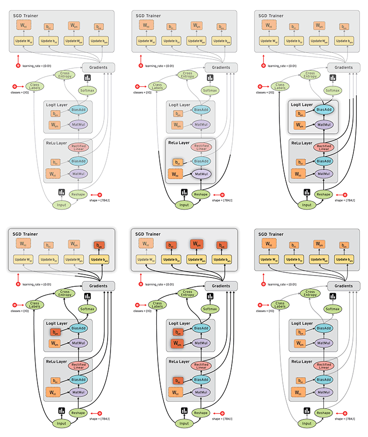
TensorFlow is an open source software library for numerical computation using data flow graphs. Nodes in the graph represent mathematical operations, while the graph edges represent the multidimensional data arrays (tensors), which communicates between them. The flexible architecture allows user to deploy computation to one or more CPUs or GPUs in a desktop, server, or mobile device with a single API. TensorFlow was originally developed by researchers and engineers working on the Google Brain Team within Google's Machine Intelligence research organization for the purposes of conducting machine learning and deep neural networks research, but the system is general enough to be applicable in a wide variety of other domains as well. Read this wiki page, you will be able to:
- know how TensorFlow works,
- build a simple, basic neural network,
- build a convolutional neural network.
This wiki-page start from very simple principle of deep learning, there will be some notation after every code we write, which is very friendly to the beginners.
Citation:
The original author for Basic Usage and MNIST tutorial is the team of TensorFlow, you can find the link of the page here: Tensorflow. But we add a lot of our things to the tutorial to make the reader more easily understand how to use TensorFlow. We test the code provided by TensorFlow team, and we correct the error in the code, we write the commands to explain the meaning behind. TensorFlow doesn't provided the code for user, to tell them how to use the visualization tool TensorBoard, so we write the code to tell the reader, how to visualize the architecture of the network and how to record the important information, like loss, the change of weights and biases for each layer.
Basic Usage
TensorFlow is a programming system in which you represent computations as graphs. Nodes in the graph are called operations. An operation takes zero or more Tensors, performs some computation, and produces zero or more Tensors. In TensorFlow terminology, a Tensor is a typed multi-dimensional array. For example, you can represent a mini-batch of images as a 4-D array of floating point numbers with dimensions [batch, height, width, channels]. A TensorFlow graph is a description of computations. To compute anything, a graph must be launched in a Session. A Session places the graph ops onto Devices, such as CPUs or GPUs, and provides methods to execute them. The technology of TensorFlow can be summarized:
- Represents computations as graphs.
- Executes graphs in the context of
Sessions. - Represents data as tensors.
- Maintains state with
Variables. - Uses feeds and fetches to get data into and out of arbitrary operations.
Building the graph
To build a graph start with operations that do not need any input, such as Constant, and pass their output to other ops that do computation.
import tensorflow as tf
graph = tf.Graph()
with graph.as_default():
matrix = tf.constant([[3., 3.]]) # create a constant 1x2 matrix
matrix = tf.constant([[2.],[2.]]) # create a constant 2x1 matrix
product = tf.matmul(matrix1,matrix2) # creat a Matmul op that takes 'matrix1' and 'matrix2' as inputs
The default graph now has three nodes: two constant() operations and one matmul(), to actually multiply the matrices and get the result of the multiplication, you must launch the graph in a session.
Launching the graph in a session
You need create a Session object, to laugh a graph. Without arguments the session constructor launches the default graph.
with tf.Session() as sess:
  with tf.device("/gpu:1"):
    matrix1 = tf.constant([[3., 3.]])
    matrix2 = tf.constant([[2.],[2.]])
    product = tf.matmul(matrix1, matrix2)
The Session closes automatically at end of this block. If you have more than one GPU available on your machine, to use a GPU beyond the first you must assign ops to it explicitly. Devices are specified with strings. The currently supported devices are:
"/cpu:0": The CPU of your machine."/gpu:0": The GPU of your machine, if you have one."/gpu:1": The second GPU of your machine, etc.
Variables
Variables maintain state across executions of the graph. The following example shows a variable serving as a simple counter, to count number from 1 to 10:
# Create a Variable, that will be initialized to the scalar value 0.
state = tf.Variable(0, name="counter")

# Create an Op to add one to `state`.

one = tf.constant(1)
new_value = tf.add(state, one)
update = tf.assign(state, new_value)

# Variables must be initialized by running an `init` Op after having
# launched the graph.  We first have to add the `init` Op to the graph.
init_op = tf.global_variables_initializer()

# Launch the graph and run the ops.
with tf.Session() as sess:
  # Run the 'init' op
  sess.run(init_op)
  # Print the initial value of 'state'
  print(sess.run(state))
  # Run the op that updates 'state' and print 'state'.
  for _ in range(10):
    sess.run(update)
    print(sess.run(state))
Fetches and Feeds
To fetch the outputs of operations, execute the graph with a run() call on the Session object and pass in the tensors to retrieve. In the previous example we fetched the single node state, but you can also fetch multiple tensors:
input1 = tf.constant([3.0])
input2 = tf.constant([2.0])
intermed = tf.add(input1, input2)
mul = tf.mul(input1, intermed)

with tf.Session() as sess:
  result = sess.run([mul, intermed])
  print(result)
A feed temporarily replaces the output of an operation with a tensor value. You supply feed data as an argument to a run() call. The feed is only used for the run call to which it is passed. The most common use case involves designating specific operations to be "feed" operations by using tf.placeholder() to create them:
input1 = tf.placeholder(tf.float32)
input2 = tf.placeholder(tf.float32)
output = tf.mul(input1, input2)

with tf.Session() as sess:
  print(sess.run([output], feed_dict={input1:[7.], input2:[2.]}))
MNIST Tutorial
This tutorial is intended for readers who are new to both machine learning and TensorFlow, when one learns how to program, there's a tradition that the first thing you do is print "Hello World." Just like programming has Hello World, deep learning has MNIST. MNIST is a simple computer vision dataset, it consists of images of handwritten digits like this:
In this tutorial, we're going to train a model to look at images and predict what digits they are.
The MNIST Data
The MNIST data is hosted on Yann LeCun's website.
The MNIST data is split into three parts: 55,000 data points of training data (mnist.train), 10,000 points of test data (mnist.test), and 5,000 points of validation data (mnist.validation). This split is very important: it's essential in machine learning that we have separate data which we don't learn from so that we can make sure that what we've learned actually generalizes.
As mentioned earlier, every MNIST data point has two parts: an image of a handwritten digit and a corresponding label. We'll call the images "x" and the labels "y". Both the training set and test set contain images and their corresponding labels; for example the training images are mnist.train.images and the training labels are mnist.train.labels.
Each image is 28 pixels by 28 pixels. We can interpret this as a big array of numbers:
We can flatten this array into a vector of 28x28 = 784 numbers. The result is that mnist.train.images is a tensor (an n-dimensional array) with a shape of [55000, 784]:
Each image in MNIST has a corresponding label, a number between 0 and 9 representing the digit drawn in the image. For the purposes of this tutorial, we're going to convert our labels as "one-hot vectors". A one-hot vector is a vector which is 0 in most dimensions, and 1 in a single dimension. In this case, the n-th digit will be represented as a vector which is 1 in the nth dimension. For example, 3 would be [0,0,0,1,0,0,0,0,0,0]. Consequently, mnist.train.labels is a[55000, 10] array of floats.
We're now ready to actually make our model.
Soft-max Regressions
We know that every image in MNIST is of a handwritten digit between zero and nine. So there are only ten possible things that a given image can be. We want to be able to look at an image and give the probabilities for it being each digit. For example, our model might look at a picture of a nine and be 80% sure it's a nine, but give a 5% chance to it being an eight (because of the top loop) and a bit of probability to all the others because it isn't 100% sure.
If you want to assign probabilities to an object being one of several different things, soft-max is the thing to do, because soft-max gives us a list of values between 0 and 1 that add up to 1. A soft-max regression has two steps:
- we add up the evidence of our input being in certain classes
- we convert that evidence into probabilities.
The result is that the evidence for a class i given an input x is:
| \text{evidence}_i = \sum_j W_{i,~ j} x_j + b_i |
where W_i is the weights and b_i is the bias for class i, and j is an index for summing over the pixels in our input image x. We then convert the evidence tallies into our predicted probabilities y using the "soft-max" function:
| prediction = \text{softmax}(\text{evidence}) |
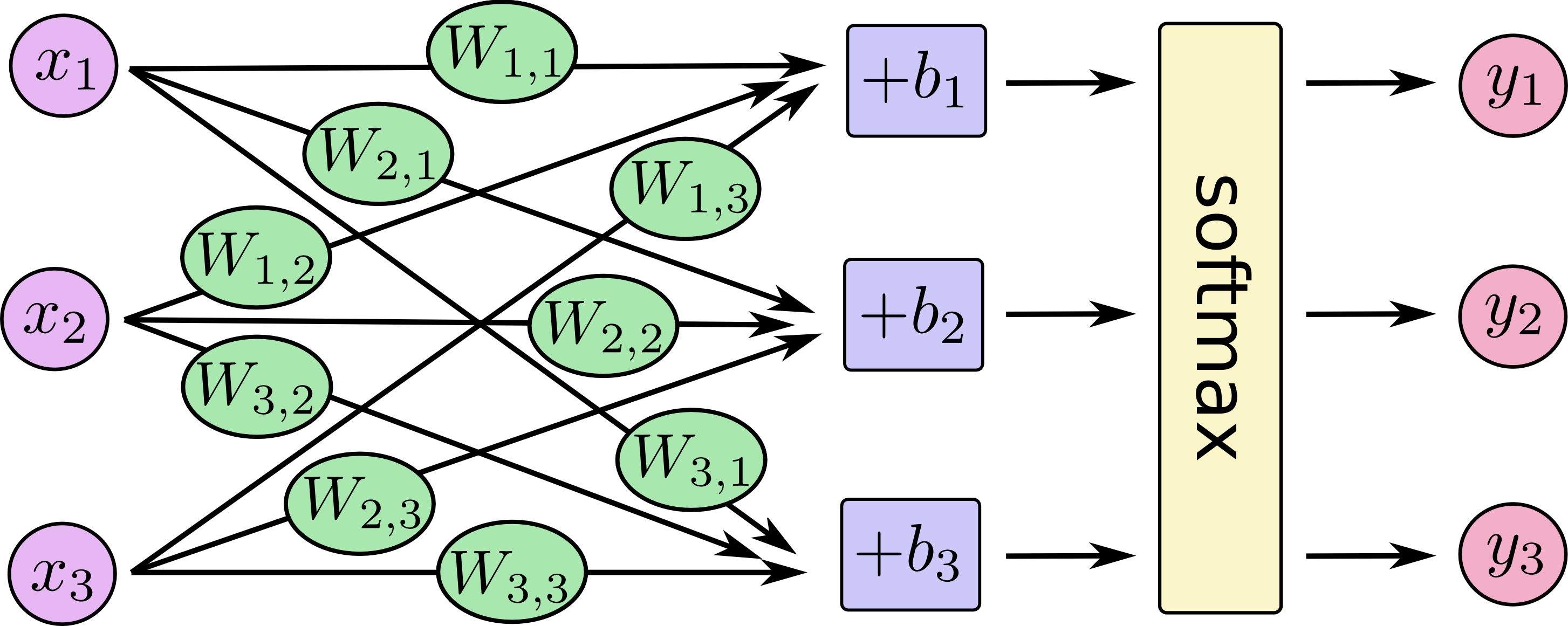
You can picture our soft-max regression as looking something like the following, although with a lot more x_i. For each output, we compute a weighted sum of the x_i, add a bias, and then apply soft-max.
More compactly, we can just write:
| prediction = \text{softmax}(Wx + b) |
Now let's implement this model in TensorFlow.
Implementation
This is code wirten with the programming language python-2.7, the accuracy of classification of the digit number after training is about 92%.
import tensorflow as tf #To use TensorFlow, first we need to import it
from tensorflow.examples.tutorials.mnist import input_data
mnist = input_data.read_data_sets("MNIST_data/", one_hot=True) # download and read in the MNIST data
x = tf.placeholder(tf.float32, [None, 784])
y = tf.placeholder(tf.float32, [None, 10]) # We will input a value for x and y when we ask TensorFlow to run a computation. We want to be able to input any number of MNIST images, each flattened into
a 784-dimensional vector. We represent this as a 2-D tensor of floating-point numbers, with a shape [None, 784].
(Here None means that a dimension can be of any length)
W = tf.Variable(tf.zeros([784, 10]))
b = tf.Variable(tf.zeros([10])) # A Variable is a modifiable tensor that lives in TensorFlow's graph of interacting operations. We use Variables to define the weights and biases
prediction = tf.nn.softmax(tf.matmul(x, W) + b) # implement our model
cross_entropy = tf.reduce_mean(-tf.reduce_sum(y * tf.log(prediction), reduction_indices=[1])) # cross-entropy is measuring how inefficient our predictions are for describing the truth. The cross-entropy is defined as the loss function
train_step = tf.train.GradientDescentOptimizer(0.5).minimize(cross_entropy) # we ask TensorFlow to minimize cross_entropy using the gradient descent algorithm with a learning rate of 0.5
correct_prediction = tf.equal(tf.argmax(y, 1), tf.argmax(prediction, 1)) # One last thing before we launch it, we have to create an operation to initialize the variables we created
accuracy = tf.reduce_mean(tf.cast(correct_prediction, tf.float32)) # calculate the accuracy of prediction
for i in range(1000): # We can now launch the model in a Session, and train it 1000 times
with tf.Session() as sess:
tf.initialize_all_variables().run()
batch_xs, batch_ys = mnist.train.next_batch(100)
sess.run(train_step, feed_dict={x: batch_xs, y: batch_ys})
print(sess.run(accuracy, feed_dict={x: mnist.test.images, y: mnist.test.labels})) # Evaluate the model with test data, that gives us a list of booleans. To determine what fraction are correct, we cast to floating point numbers
and then take the mean. For example, [True,False, True, True] would become [1,0,1,1] which would become 0.75.
you can find the full code from this link: Example 1
Implementation of convolutional neural network for MNIST data
Getting 92% accuracy on MNIST is bad. It's almost embarrassingly. In this section, we'll fix that, jumping from a very simple model to something moderately sophisticated: a small convolutional neural network. This will get us to around 99.2% accuracy -- not state of the art, but respectable.
Weight Initialization
To create this model, we need to create a lot of weights and biases. One should generally initialize weights with a small amount of noise for symmetry breaking, and to prevent 0 gradients. Since we're using ReLU neurons, it is also good practice to initialize them with a slightly positive initial bias to avoid "dead neurons". Instead of doing this repeatedly while we build the model, let's create two handy functions to do it for us.
def weight_variable(shape):
  initial = tf.truncated_normal(shape, stddev=0.1)
  return tf.Variable(initial)

def bias_variable(shape):
  initial = tf.constant(0.1, shape=shape)
  return tf.Variable(initial)
Convolution and Pooling
TensorFlow also gives us a lot of flexibility in convolution and pooling operations. Our convolutions uses a stride of one and are zero padded so that the output is the same size as the input. Our pooling is plain old max pooling over 2x2 blocks. To keep our code cleaner, let's also abstract those operations into functions.
def conv2d(x, W):
  return tf.nn.conv2d(x, W, strides=[1, 1, 1, 1], padding='SAME')

def max_pool_2x2(x):
  return tf.nn.max_pool(x, ksize=[1, 2, 2, 1], strides=[1, 2, 2, 1], padding='SAME')
First Convolutional Layer
We can now implement our first layer. It will consist of convolution, followed by max pooling. The convolution will compute 32 features for each 5x5 patch. Its weight tensor will have a shape of [5, 5, 1, 32]. The first two dimensions are the patch size, the next is the number of input channels, and the last is the number of output channels. We will also have a bias vector with a component for each output channel.
W_conv1 = weight_variable([5, 5, 1, 32])
b_conv1 = bias_variable([32])
To apply the layer, we first reshape x to a 4d tensor, with the second and third dimensions corresponding to image width and height, and the final dimension corresponding to the number of color channels.
x_image = tf.reshape(x, [-1,28,28,1])
We then convolve x_image with the weight tensor, add the bias, apply the ReLU function, and finally max pool. The max_pool_2x2 method will reduce the image size to 14x14.
h_conv1 = tf.nn.relu(conv2d(x_image, W_conv1) + b_conv1)
h_pool1 = max_pool_2x2(h_conv1)
Second Convolutional Layer
In order to build a deep network, we stack several layers of this type. The second layer will have 64 features for each 5x5 patch.
W_conv2 = weight_variable([5, 5, 32, 64])
b_conv2 = bias_variable([64])

h_conv2 = tf.nn.relu(conv2d(h_pool1, W_conv2) + b_conv2)
h_pool2 = max_pool_2x2(h_conv2)
Densely Connected Layer
Now that the image size has been reduced to 7x7, we add a fully-connected layer with 1024 neurons to allow processing on the entire image. We reshape the tensor from the pooling layer into a batch of vectors, multiply by a weight matrix, add a bias, and apply a ReLU.
W_fc1 = weight_variable([7 * 7 * 64, 1024])
b_fc1 = bias_variable([1024])

h_pool2_flat = tf.reshape(h_pool2, [-1, 7*7*64])
h_fc1 = tf.nn.relu(tf.matmul(h_pool2_flat, W_fc1) + b_fc1)
Dropout
To reduce overfitting, we will apply dropout before the readout layer. We create a placeholder for the probability that a neuron's output is kept during dropout. This allows us to turn dropout on during training, and turn it off during testing. TensorFlow's tf.nn.dropout op automatically handles scaling neuron outputs in addition to masking them, so dropout just works without any additional scaling.
keep_prob = tf.placeholder(tf.float32)
h_fc1_drop = tf.nn.dropout(h_fc1, keep_prob)
Readout Layer
Finally, we add a layer, just like for the one layer softmax regression above.
W_fc2 = weight_variable([1024, 10])
b_fc2 = bias_variable([10])

prediction = tf.matmul(h_fc1_drop, W_fc2) + b_fc2
Train and Evaluate the Model
To train and evaluate it we will use code that is nearly identical to that for the simple one layer SoftMax network above.
The differences are that:
We will replace the steepest gradient descent optimizer with the more sophisticated ADAM optimizer.
We will include the additional parameter
keep_probinfeed_dictto control the dropout rate.We will add logging to every 100th iteration in the training process.
cross_entropy = tf.reduce_mean(tf.nn.softmax_cross_entropy_with_logits(prediction, y))
train_step = tf.train.AdamOptimizer(1e-4).minimize(cross_entropy)
correct_prediction = tf.equal(tf.argmax(y_conv,1), tf.argmax(y_,1))
accuracy = tf.reduce_mean(tf.cast(correct_prediction, tf.float32))
with tf.Session() as sess:
    tf.initialize_all_variables().run()
    for i in range(20000):
      batch = mnist.train.next_batch(50)
      if i%100 == 0:
        train_accuracy = accuracy.eval(feed_dict={x:batch[0], y: batch[1], keep_prob: 1.0})
        print("step %d, training accuracy %g"%(i, train_accuracy))
      train_step.run(feed_dict={x: batch[0], y: batch[1], keep_prob: 0.5})
    print("test accuracy %g"%accuracy.eval(feed_dict={x: mnist.test.images, y: mnist.test.labels, keep_prob: 1.0}))
The final test set accuracy after running this code should be approximately 99.2%. The full code you can see from this link Example 2.
Serializing the data
TensorBoard operates by reading TensorFlow events files, which contain summary data that you can generate when running TensorFlow. Here's the general life-cycle for summary data within TensorBoard.
First, create the TensorFlow graph that you'd like to collect summary data from, and decide which nodes you would like to annotate with summary operations.
For example, suppose you are training a convolutional neural network for recognizing MNIST digits. You'd like to record how the learning rate varies over time, and how the objective function is changing. Collect these by attaching scalar_summary ops to the nodes that output the learning rate and loss respectively. Then, give each scalar_summary a meaningful tag, like 'learning rate' or 'loss function'.
Perhaps you'd also like to visualize the distributions of activation coming off a particular layer, or the distribution of gradients or weights. Collect this data by attaching histogram_summary ops to the gradient outputs and to the variable that holds your weights, respectively. Operations in TensorFlow don't do anything until you run them, or an op that depends on their output. And the summary nodes that we've just created are peripheral to your graph: none of the ops you are currently running depend on them. So, to generate summaries, we need to run all of these summary nodes. Managing them by hand would be tedious, so use tf.summary.merge_all to combine them into a single op that generates all the summary data.
Then, you can just run the merged summary op, which will generate a serialized Summary protobuf object with all of your summary data at a given step. Finally, to write this summary data to disk, pass the summary protobuf to a tf.train.SummaryWriter. The SummaryWriter takes a logdir in its constructor - this logdir is quite important, it's the directory where all of the events will be written out. Also, the SummaryWriter can optionally take a Graph in its constructor. If it receives a Graphobject, then TensorBoard will visualize your graph along with tensor shape information.
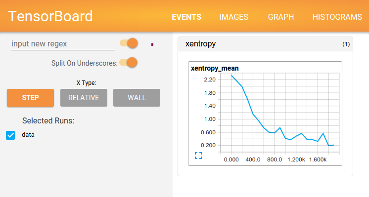
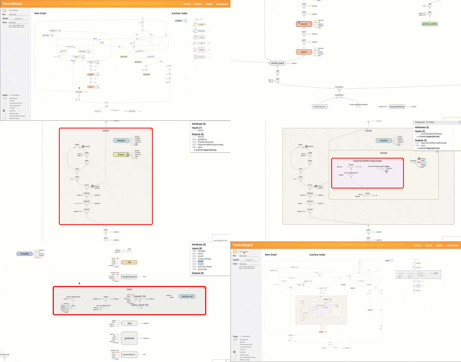
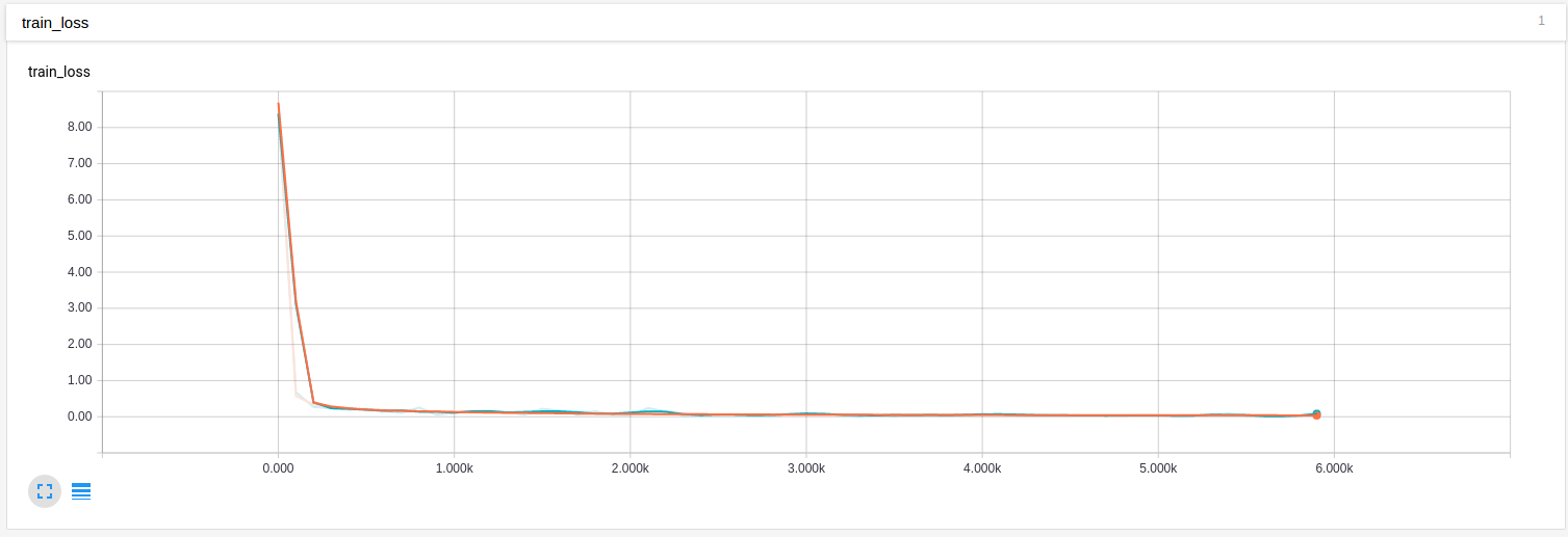
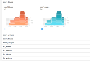
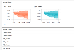
The Example 3 example is a modification of the implementation of convolutional neural network for MNIST data above, this code show how to record the loss or the change of weights and biases mentioned above. The results are illustrated in the figures below:
The loss
Visualization of Graph
The change of weights and biases
Launching TensorBoard
To run TensorBoard, use the following command in a terminal:
tensorboard --logdir=logs
And open the link in a web-page.
Weblinks
https://www.tensorflow.org/ (Tensorflow Homepage)
https://en.wikipedia.org/wiki/TensorFlow (Wikipedia Tensorflow)

